WIXLIB

2.2. C HOICE OF T URBULENCE MODEL5able for many flows and easy to implement. This equation is valid for fully turbulentflows. However, the prediction is poor for strong separation and rotational flows.There is also k- RNG model which gives good prediction only for transition flows.k- ωThis model is based on turbulent kinetic energy (k) and length scale (ω) rather thandissipation rate and the main advantage is no changes are required to integrate nearthe wall in the viscous sublayer.2.2.47 equation modelThis model solves Reynolds stress and equation. This model has no isotropicassumptions and it is better as turbulence is different in different directions. Thisis more complete but it requires six additional equations for each of the turbulentstresses and an equation for . Therefore, computational effort is large and thepartial differential equations are very stiff. The results are not much better than 1 or2 equations model to justify extra computational effort.2.2.5Shear Stress Transport (SST) modelThis combines both the two equation models k- and k-ω. With k-ω it can modelviscous sublayer and switches to k- in the free stream and avoids sensitivity of k-ωmodel.The turbulent boundary layer can be sub-divided into three layers. The laminar sublayer (layer close to wall), the log layer and the outer layer. To resolve the boundarylayer there are two approaches as to either use a wall function correlation (30 y 300) which is empirical or use y 1. The y is a non-dimensional normal spacingfrom the airfoil surface whose value determines the part of turbulent boundary layerthat needs to be resolved. The first method of using standard wall function is goodfor high Reynolds number flows as the case under consideration. This method resolves the log layer where there is equilibrium between production and dissipation ofturbulent energy and therefore avoids the turbulent instabilities in near wall analysisin viscous sub layer. By this method the order of resolving the boundary layer canbe reduced to 102 compared with the usage of y 1. However, in the separationregion wall function does not give good approximation. Though the second methodof resolving y 1 is computationally expensive, it gives very good refinement of thesublayer close to the wall and works fine for complex flows and flows involving separation. Hence for the analysis here SST turbulent model is utilised with y 1 forresolving boundary layer.

6C HAPTER 2. S ELECTION OF TURBULENCE SCHEME AND NUMERICAL PARAMETERS2.3Spatial discretisationIn order to resolve Navier-Stokes equations, both the spatial and time domain needto be discretised. To resolve the spatial domain, it is necessary to define numericalschemes for the flow variables.For the compressible flows, shock and rarefraction waves appear naturally and theyare well described as Riemann problem. While resolving the hyperbolic part ofNavier-Stokes equation various schemes were established to solve the Riemannproblem for high schock resolution and reduce the oscillations. To solve the appropriate Riemann problem, Godunov linear method or non-linear TVD schemes canbe used. But they are of 1st order and 2nd order respectively. Hence in order toget accurate and smooth results for the Riemann problem it is necessary to makehigher order schemes. However, the exact solution of the Riemann problem becomes expensive and practically unusable for complex problems. The higher orderschemes like Roe, JST, etc., which are approximate Riemann solvers which containmore physical information of the flow can be used as these are computationally efficient and accurate. The incompressible flow approximation in SU2 adopts artificialcompressibility for pressure and velocity decoupling and so the already establishedsolutions of the Riemann problem to resolve compressible flow variables can be employed for incompressible flows (Kong [2011]). The JST schemes is more stable butrequires finer mesh compared to ROE scheme to attain same order of accuracy.Hence in the analysis of flow variables, ROE scheme has been used.To solve the spatial gradients Weighted Least Square (WLS) or Green Gauss (GG)numerical methods can be used in SU2. WLS avoids the error from the outliersand its performance is good for structured meshes. The GG method has low errors for triangular and quadrilateral cells. Here in all the cases under consideration,the meshes are structured and so both the type of slope limiter works good. Although the higher order schemes discussed above give good approximations, theysometimes introduce unphysical wiggles and so flux limiters are used. The Minmodlimiter is a conservative reconstruction with minimum slope available. This is themost diffusive of all the limiters and least accurate. The Superbee limiter on theother hand has five segments in it and follows the upper boundary of the viable limiter. This has the steepest slope possible and does not yield good result for smoothflows. Therefore in SU2 analysis, Venkatakrishnan limiter is used which is smoothand continuous and lies between Minmod, Superbee limiters.

2.4. T IME DISCRETISATION SCHEME2.47Time discretisation schemeThe available time discretisation schemes in SU2 are implicit, explicit Euler andRunge-kutta schemes. The choice of the scheme for time discretisation is implicitEuler schemes. Though the implicit scheme has one additional step of computation,higher CFL can be used which facilitates faster convergence without blowing up thesolution convergence and accuracy. This justifies the extra computational effort itrequires.

8C HAPTER 2. S ELECTION OF TURBULENCE SCHEME AND NUMERICAL PARAMETERS

Chapter 3DU97-W-300 AirfoilOne of the airfoils considered for analysis is TU Delft DU97-W-300, non-symmetricand blunt trailing edge airfoil with 30% thickness and 0.65 m of chord length. The experimental values are taken from the Avatar project, (Manolesos and Prospathopoulos [2015]) for this airfoil to compare with the results from SU2. The experimentis performed in low speed low turbulent wind tunnel with the Reynolds number of2.106 . The lift and drag coefficients from SU2 is compared with the correspondingplots from the experiment and with the results from other computational platformslike MapFlow, Q3UIC, Rfoil and Xfoil.The MapFlow is a compressible solver adopted with pre-conditioning for low Machnumber (incompressible) flows. The discretisation used is cell centred ROE schemefor convection term with Venkatakrishnan limiter. The turbulence model used isSST and time discretisation is implicit second order method. The schemes used inMapFlow is similar to that being used in SU2 for analysis as described in the previous section.The Q3UIC Quasi-three dimensional Unsteady viscous-inviscid Interaction Code isdeveloped to predict wind turbine aerodynamic performance. The inviscid part ismodelled by a panel method and the viscous part is modelled by solving the integralform of the equations. Here the tripping of the laminar to boundary layer is done byeither boundary layer tripping or by en transition method.Xfoil and Rfoil are engineering models for aerodynamics design of airfoils. Rfoilis an in-house tool developed by ECN based on Xfoil with additional rotational effects and gives good prediction for thick airfoils. Here the analysis with SU2, Xfoiland Rfoil are performed for fully turbulent flows whereas the experiment and othernumerical tools involve transition flow.9

103.1C HAPTER 3. DU97-W-300 A IRFOILEvaluation of boundary layer to generate meshThe main idea is to resolve the boundary layer to get better predictions for separated flows. Hence reasonable prediction of boundary layer thickness is estimatedfrom Xfoil for various angles of attack. The mesh is generated based on the estimation from Xfoil tripped cases. The separation point for each angle of attack isestimated from Xfoil tripped cases and the mesh is refined based on the y 1 insidethe boundary layer. The separation point is calculated based on the skin frictioncoefficient (Cf ) and the shape factor H (H is the ratio of displacement thickness tomomentum thickness). Cf decreases drastically during transition and increases asthe flow become turbulent due to increase in shear stress. Eventually Cf becomeszero when the flow separates. Further, H increases and then decreases as the flowchanges from transition to turbulent due to the sudden increase in the displacementthickness. The shape factor reaches the maximum value of about 1.3 and thendips indicating the point of separation where the displacement thickness increasesrapidly. Therefore, the position along the airfoil where H becomes maximum and Cfbecome zero indicates the flow separation.Figure 3.1: Boundary layer thickness extracted from Xfoil simulationsFigure 3.1 shows the plot of boundary layer thickness along the suction and pressure side of the airfoil for angle of attack 8, 12 and 16 degrees. The boundary layerthickness is shown only for region of non-separated flow. It can be seen that theseparation starts at 12-degree angle of attack at x 0.55. Based on the boundarylayer analysis from the above figures, the maximum boundary layer thickness thatcan be reached is 0.06 which is a normalised by the chord length. From the chordlength of 0.65m it can be found that the maximum boundary layer thickness is 32.5mm and so the mesh is resolved finer for this thickness and a growth rate of less

3.2. L IFT- COEFFICIENT11than 1.2 is maintained in the region normal to it. The boundary layer is resolved withy 1 as this gives a good result for separated flows and double precision is usedto avoid round off errors. Four different meshes used for the analysis which are 300surface points on airfoil with 300 normal points, 500 surface points with 450 normalpoints, 500 surface points with 600 normal points and 1000 surface points with 1000normal points.3.2Lift-coefficientFigure 3.2: Comparison of lift coefficient obtained by various numerical methodsand experimental dataThe plot of lift coefficient versus Angle of Attack (AoA) is shown in the figure 3.2.The results for the four meshes overlap on each other indicating a grid independentsolution. The experimental data and the Mapflow result involves transition and sothey predict higher lift coefficient (Cl ) values than the corresponding AoA from othernumerical tools. The Cl from SU2 are comparatively lower than non-tripped casesbut stalls at around the same position. This is due to the influence of thicker boundary layer for turbulent flows where the velocity deficit is large which eventually leadsto less difference in freestream and local pressure (δP ) and hence lower lift.Rfoil is known to be more accurate for thick airfoils and so the result from SU2 iscompared with Rfoil tripped cases. It is found that the SU2 over predicts to a maximum of 5% in the linear region and over prediction increases in the stall regionto around 30%. However, in deep stalled region (i.e. 20 degrees angle of attack),the results from SU2 lies closer to Rfoil tripped scenario. At the same time, it is to

12C HAPTER 3. DU97-W-300 A IRFOILbe noted that the performance of SU2 in stall is relatively better than Q3UIC panelmethod.3.3Drag-coefficientFigure 3.3: Comparison of drag coefficients obtained by various numerical methodsand experimental data.Figure 3.3 shows the plot of drag for various angle of attack. The drag has twoparts namely skin friction drag and pressure drag. Generally, the skin friction dragis more predominant over the airfoils. However, as flow separates the pressure drag(form drag) increases thus causing the overall drag to increase. The reason for thegeneral trend of increase in drag coefficient as AoA increases. Here, as SU2 andRfoil involves tripped flow (fully turbulent) the drag coefficient is comparatively higherthan that of Mapflow and experiment. However, the drag coefficient calculated fromSU2 is under predicting than that of Rfoil tripped case throughout the entire domainof Aoa -5 to 16 degrees. This underprediction grows when the flow gets separated.

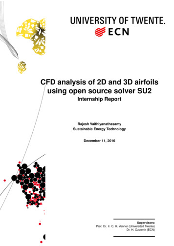
3.4. P RESSURE COEFFIICENT (Cp )3.413Pressure coeffiicent (Cp)(a) AoA -4(b) AoA 0(c) AoA 4(d) AoA 8(e) AoA 12(f) AoA 16Figure 3.4: Comparison of Cp for the various angle of attacks between SU2 andRfoil tripped cases.Figure 3.4 shows the comparison of the plot of Cp from SU2 with that of the Rfoiltripped cases for all angle of attacks considered in the polar above. The positionof the lowest pressure at the suction side can be seen moving towards the leadingedge as the AoA increases. This indicates the increase in the adverse pressuregradient. Also the Cp is over predicted compared to the Rfoil tripped case for allAoAs. The separation for 12 and 16 degrees AoA can be clearly seen as indicated bythe negligible changes in the pressure coefficient in the suction side as x/c increases.However, the separation is predicted at a later position of x/c in comparison with Rfoiltripped case.

14C HAPTER 3. DU97-W-300 A IRFOIL

Chapter 4FFA-W3-301 AirfoilThe airfoil under consideration is FFA-W3-301 which is being used in wind turbines.It has a chord length of 0.6 m with thickness of 30% and it is tested at Reynoldsnumber of 1.6 million in laminar wind tunnel of Stuttgart University. The numericalanalysis of airfoil is carried out and compared for fully turbulent flows. Turbulentflows produce more drag compared to laminar flows. However, the flow is stableand the small disturbances are damped out whereas it is not the case with the laminar flows. Hence even if the drag is higher for turbulent flows, it is preferred for thereliable performances sacrificing little efficiency. As SU2 is used for turbulent analysis, the airfoil experimental data (P. Fuglsang and Madsen [1998]) with leading edgeroughness (LER) is taken as a benchmark to compare the results. To obtain LEReffect, trip tape is used in experiments. LER is generally observed when dirt is accumulated while operating the wind turbine in dirty environment. The SU2 analysis isdone at the same Reynolds number of 1.6 million and validated with the experimentand the Navier-Stokes solver Ellipsys 2D for turbulent flow conditions. The Xfoil andRfoil tripped cases are also considered for comparison. Tripping of Xfoil and Rfoilis done at x/c 0.05 from the leading edge both on pressure side and suction side.The value of x/c for tripping in both Xfoil and Rfoil is chosen in such a way that thestagnation point remains just before the tripping point even at very high angle ofattack. Since the airfoil under consideration is very thick, Rfoil tripped scenario isconsidered a very good benchmark to compare the SU2 results.4.1Mesh Generation2D structured O-mesh is used for the analysis. Structured mesh offers simplicityand easy data access. The element choice is quadrilateral as this is highly efficientto get good convergence and high resolution. The boundary layer is refined withy 1. The wall spacing s is calculated based on, (Schlichting [1979]) :15

16C HAPTER 4. FFA-W3-301 A IRFOILδs y ν/ρu ,(4.1)where ρ is the density of air, µ is the dynamic viscosity and u is the friction velocity. The density and dynamic viscosity are taken at the conditions of standardtemperature and pressure. The friction velocity is given bypu τw /ρ,(4.2)where, τw 0.5Cf ρ U 2 ,Cf 0.0576 Rex 1/5f or 5 · 105 Rex 107 ,with y the wall spacing δs is calculated to be 8.5 · 10 6 . The wall spacing is givenas the constraint at the boundary layer. The far field is fixed at 90 times the chordlength for minimizing the effect of boundary conditions on calculated flow variables.The O-mesh is preferred due to its larger stability at the trailing edge for high gradient flows (Lutton [1989]). This is due to the large accumulation of grid points nearthe trailing edge which facilitates smooth gradient transformation. The O-mesh alsoallows better estimation of angle of attack at Clmax . The skewness of the mesh iskept under 0.67 and the area ratio between the cells around a maximum of 1.4. Theaspect ratio which is the ratio of length to width is kept under 4000. The larger values of the above properties than prescribed leads to convergence problem and badinterpretation of the result.Figure 4.1 shows the mesh generated as per the above mentioned parameter with300 points on the airfoil surface and 400 points normal to it. On performing simulation, it is found that in some points the y exceeds 1 even though the wall spacingof 8.5 · 10 6 used in the mesh is calculated theoretically using y 1.

4.1. M ESH G ENERATIONFigure 4.1: Mesh with approximately 120000 cells17

184.2C HAPTER 4. FFA-W3-301 A IRFOILFinding the right wall spacing:Figure 4.2: y for theoretical and altered wall spacingFigure 4.2 shows the plot of y versus dimensionless x-coordinate of the airfoilfor the previously shown mesh at 10 degrees angle of attack. The theoreticallycalculated wall spacing of 8.5 · 10 6 for y 1 yields y value of 1.8 at the suctionside of the airfoil near the leading edge. Even though the calculated wall spacingutilises the local Reynolds number, this higher value of y at the leading edge is dueto the high angle of attack which is not taken into account while calculating the wallspacing. In order to get the y less than 1 even at higher angle of attack, the wallspacing is linearly reduced to 3.5 · 10 6 for which the y remains less than 1 aroundthe entire airfoil as shown in the figure as altered wall spacing.Figure 4.3: Comparison of Cp for theoretical and altered wall spacing with experiment

4.3. S TEADY AND U NSTEADY SIMULATION19Figure 4.3 shows the plot of pressure coefficient (Cp ) versus dimensionless xcoordinate from the SU2 analysis for the same mesh. This includes the results forcalculated and altered wall spacing along with the experimental values for angle ofattack of 10 degrees. At this angle of attack the flow begins to separate as evidentfrom the experimental data where the change in pressure coefficient is very littletowards the trailing edge beyond x/c 0.6. Also SU2 predicts the separation butat a farther position in the chord at x/c 0.83. At this point the change in pressurecoefficient starts to become insignificant. The separation is almost at the same pointfor both theoretically calculated δs and corrected δs. However, for the corrected wallspacing the Cp distribution lies closer to the experimental value. Hence the correctedwall spacing of 3.5 · 10 6 is utilised in the remaining analysis.4.3Steady and Unsteady simulationBoth the steady and unsteady simulations are performed to compare the result withthe experimental data. The steady state simulation is based on the method previously described with the choice of turbulence model as SST. Further the unsteadysimulation is carried out to check for the improvement of the solution. For the unsteady simulation, dual time stepping is used to achieve faster convergence. Implicitmethod can also be used which retains higher order of accuracy. This facilitateslarger time step without affecting the solution convergence. But the usage of implicitmethod is expensive for both 2D and 3D cases as it involves large number of pointsand require huge system of equations to solve. Therefore dual time stepping is preferred.While solving the Navier-Stokes equations, the momentum equation is uncoupledas velocity and pressure terms and solved separately. The velocity is calculated asan intermediate step followed by the pressure in the next time step. Finally the velocity is corrected in 3rd step. This method of solving is 1st order pressure accurateas pressure is completely dis

The open source computational fluid dynamics (CFD) software SU2 is developed for compressible flows, equipped with approximations like pre-conditioning and artificial compressibility for incompressible flows. Wind turbines operate at very low velocity and is a good example of incompressible flows. The performance of SU2 at these