Transcription
1Economic Comparison of aSimulator-Based GLR Methodfor Pipeline Leak Detectionwith Other MethodsEric Penner, Josh Stephens, Elijah Odusina, James Akingbola,David Mannel and Miguel BagajewiczDepartment of Chemical Engineering and Materials ScienceUniversity of Oklahoma1
2AbstractIn this paper, we show a simulator-based implementation of the Generalized LikelihoodRatio method to detect leaks and locate biases in pipelines. We compare its leak detectionability, costs, and levels of tuning required to those of other software and hardware leakdetection methods. The economic comparison includes computing the losses for not detectingthe leaks. It was found that GLR is the most economic leak detection method available.Simulations were run with varying pipe diameters, price of oil, and cost of leak clean up.2
3IntroductionPipelines are the most commonly used method to deliver petroleum products, naturalgas, liquid hydrocarbons, and water to consumers. The petroleum pipeline network in theUnited States transports over 600 billion ton-miles of freight each year. It accomplishes this jobin an exceptionally effective manner. In fact, oil pipelines transport 17% of all US freight butcost only 2% of the freight bill. They do so in a cost effective and safe manner; however, safetyand losses due to leaks are the number one concern in pipeline operation. The largest challengeis discovering economic leak detection methods capable of accurately detecting leaks in atimely fashion.There are three different pipeline systems: gathering systems, distribution systems, andsingle pipelines that go from one point to another. Gathering systems and distribution systemsare very similar. A gathering system has many pipes that gather the product from differentareas and funnel it into one larger pipe. A distribution system takes the product from one largepipeline and delivers it to different areas via smaller pipes. The basic idea of the two systems isthe same; the flow is simply reversed. Figure 1 illustrates the gathering and distributionnetwork system.Figure 1: Gathering/Distribution SystemsSignificant incidents for pipelines operated within the United States are tracked by theUS Department of Transportation Pipeline and Hazardous Materials Safety Administration,commonly known as the PHMSA. The number of significant incidents, including the number ofinjuries and fatalities that resulted from those incidents, has been recorded over the pasttwenty years. Figure 2 provides a graphical representation of this data. A significant incident, asdefined by the PHMSA, is a pipeline incident that meets any of the following conditions:1. A fatality or injury requiring hospitalization2. 50,000 or more in total costs, measured in 1984 dollars3. Highly volatile liquid releases of 5 barrels or more or other liquid releases of 50 barrelsor more4. Liquid releases resulting in an unintentional fire or explosion3
4Figure 2. Significant Incidents Summary 1988-2008. (Incidents,( ) Injuries,( ) Fatalities) SignificantThe causes of significant incidents and other pipeline leaks are fairly well understoodthanks to careful record keeping. The PHMSA has maintained these records for pipelinesoperated in the US. The pie chart representation in Figure 2 shows the causes of significantincidents over the past twenty years. Excavation damage is clearly the primary cause butcorrosion and material failure are close behind.Figure 3: Significant Incident Cause BreakdownPipeline spills are still small in relation to the amount of product transported. In fact,they amount to only 1 gallon per million barrel-mile, where a barrel-mile equals one barreltraveling one mile. However, leaks are expensive, both in economic and human terms. Thesignificant incident data clearly indicates that leaks do indeed injure and kill people. Theeconomic reasons for not wanting leaks can be made clear by examining the BP Alaska pipeline4
5incident that occurred in March 2006. In this case, roughly 4,800 barrels of oil were lost over afive day period and the Prudhoe Bay field later underwent a phased shut down due to the leak(BP HSE). On top of the expenses incurred from pipeline repairs and the phased shut down, theEnvironmental Protection Agency leveled a 20 million fine against the company (Loy).The paper is organized as follows: we first review the different leak detection methods,then we focus on describing our implementation of GLR and finally, we present the economiccomparison.Hardware Leak DetectionHardware leak detection methods are in general sensitive to small leak sizes and quiteaccurate regarding location. Typically, instrumentation is run along the entire length of thepipeline which helps with the detection of both large and small leaks in a timely fashion andallows for the detection of a leak anywhere along the pipeline. The instrumentation used inthese schemes also allows for an estimation of a leak’s location. This information helps tominimize both the economic and environmental impact in the event of a leak.Although significant instrumentation provides many of the advantages associated withhardware leak detection, it also provides disadvantages. The high level of instrumentationresults in installation and maintenance costs that are significant. Installation is complex,requiring a considerable amount of below surface work since many pipelines are buried.Consequently, hardware methods are commonly used for pipelines traveling through high riskareas.Acoustic EmissionThe acoustic emissions method of leak detection relies on escaping fluids giving off alow frequency acoustic signal. Acoustic sensors are placed around the entire length of pipelineto monitor the noise levels of the interior of the pipeline. A baseline or “acoustic map” of thepipeline’s acceptable noises is created. Future measurements are compared to this baselinewith any deviations outside a specified range triggering the alarm system. Once the detectionsystem has been fine tuned, false alarms are uncommon and have reportedly been as low asonce per year. The acoustic signal will be strongest near the leak, thus making it possible tolocate the leak. Typical leak detection times are 15 seconds to 1 minute, with the detectiontime being limited by the speed of sound, the distance between monitors, the datacommunication time, and the necessary computational time. The sensitivity for this type ofdetection method is 1 to 3 percent of the nominal flow for a liquid pipeline. For a pipelinecarrying gas, a hole with a diameter 2 to 10 percent that of the pipeline diameter can bedetected. The location of the leak can be estimated within 30 meters. While this method ofleak detection works well for detecting leaks large and small, it does not provide a way toestimate the size of the leak (Wavealert).5
6Monitored 1af3e56351wdaFigure 4: Acoustic Emissions MethodFiber Optic SensingThe fiber optic sensing method of leak detection utilizes fiber optic sensing probes todetect leaks. The fiber optics are placed in the soil along the pipeline and monitor thetemperature, usually recording the temperature every 0.5 meters. This temperatureinformation is achieved by analysis of scattered light using either the Raman or Brillouinscattering process as the foundation. The Raman scattering process is strictly intensity basedand was the first method proposed in the 1980’s when this technology was first used. However,in the 1990’s the Brillouin scattering process, which relies on frequency measurements and hasbeen shown to be more accurate, began to replace the Raman process and remains the toppreference to date. In the event of a leak, the escaping hydrocarbon would cause atemperature change. Gas leaks would result in a cooling of the surroundings based on the JouleThompson effect, whereas liquid leaks typically increase the temperature of the surroundingarea. A baseline profile of acceptable temperatures along the pipeline must first be obtained,but if done properly, there should be no false alarms with this method. The best sensitivityattained with this method has been 50 ml/min and leaks can be isolated based on informationfrom surrounding fiber optic probes (Nikles). If the sensors are spaced every 0.5 meters, as istypical, the location of the leak can be estimated to within a one meter range. The magnitudeand speed of the change in temperature is indicative of the fluid being transported as well asthe size of the leak (Omnisens). Although the leaks magnitude is indicated by the temperaturechange, it is still difficult to accurately predict any leaks size within a certain range. It proves tobe more an indicator of large, medium, or small. The time required to obtain a complete profileof the pipeline is dependent on the pipeline length, but typically varies between 30 seconds and5 minutes (Nikles). The price tag for this method is steep though. For a 1200 km pipeline, whichis roughly equivalent to the distance between Houston and El Paso, the material costs for thismethod can run upwards of 18 million. This does not include installation costs. So althoughfiber optics provide a very accurate method for leak detection, the initial upfront investment isconsiderable (Sensortran).Monitored Pipeline0.5 m 1wdaFiber Optic CableFigure 5: Fiber Optic Sensing Method6
7Vapor Sensing MethodWith the vapor sensing method a tube, highly permeable to the material beingtransported, is placed alongside the pipeline. A test gas is pumped through this vapor sensingtube and analyzed for vapors of the pipeline fluid. If there is a leak, the pipeline material willdiffuse through this vapor sensing tube and become apparent upon analysis. The size of theleak can be estimated based on the analysis of the gas. The larger the leak is, the higher theexpected magnitude of vapor in the tube. The mixture is transported at a flow controlled rate,making it possible to estimate the location of the leak. If done properly, the leak location can benarrowed down to 0.5% of the monitored area. For example, if a pipeline being monitored inthis manner were 10,000 meters long, the vapor sensor method could narrow down the leaklocation to a 50 meter length range of pipeline. The sensitivity of this method is 1 l/hr for liquidsand 100 l/hr for gases. Additionally, the response time usually varies from 2 to 24 hours,although this is highly dependent on pump capacity (Areva).Monitored PipelineTest GasPumpPermeable TubeVaporAnalysisFigure 6: Vapor Sensor MethodUltrasonic Flow MetersUltrasonic flow meters provide another alternative hardware leak detection method.With this method, ultrasonic flow meters are attached to the outside of the pipeline andgenerate an axial sonic wave in the pipe wall. A computer measures the time differences for thewave to travel upstream and downstream and computes the flow rate from this information.This method essentially relies on a mass flow balance which, simply stated, means the massflow rate that goes in must equal that which comes out or there is a leak (Bloom). The smallestleak that can be detected with this method is 0.5% that of the nominal flow (Controlotron).Since this operates on a mass balance, a corresponding estimate can be made regarding thesize of the leak. The leak location can only be narrowed down based on how far apart themeasurement devices are installed. For instance, if the ultrasonic flow meters are placed 50meters apart then the leak location can be narrowed down to a 50 meter range.Ultrasonic aMonitored PipelineFigure 7: Ultrasonic Flow Meter Method7
8Software Leak DetectionVolume BalanceThe first type of software leak detection considered was balancing systems. The maintypes of balancing systems are the volume balance and the compensated balance. In thevolume balance, only the flow into and out of the system are considered. The volume balanceassumes the flow in a pipeline is always at steady state, which is not necessarily true if twoliquids with different densities are mixed. Since only the inlet and outlet flow are beingconsidered in the volume balance, and third term is needed in order to compensate for changesin the line pack. Multiplying the volume balance through by the fluid’s density and adding theadditional term to account for change in the amount of fluid in the system give the followingequation:.dM(1)M I (t ) M O (t ) L 0dt.where: M I inlet mass flow rateM O outlet mass flow rateM L line packThis equation is called the compensated balance. The mass flow rate entering thesystem can be estimated from pressure and temperature readings. A leak is detected when themass of the fluid exiting the pipeline is less than the estimated mass entering the pipeline. Toaccount for the line pack, a simulation model of the pipeline has to be run. Adding the term forthe change in line pack significantly reduces the error in the volume balance. A SupervisoryControl and Data Acquisition (SCADA) system is used to control and monitor the process. Errorswill still be seen from faulty instrumentation as well as from errors in the line pack calculation(Whaley).The main problem with the volume balance method and all similar software leakdetection method is its susceptibility to false alarms in non-steady state situations. A massbalance system responds to the leak only after the pressure waves generated by the leak havetraveled to both ends of the pipeline. If there is a leak whose magnitude is less than 5% of thetotal flow, therefore, it can take on the order of few hours before the leak is detected. Thistechnique only applies to single pipelines, so complex networks like gas distribution systems inurban areas do not apply. The volume balance does not help in detecting the location of leaks,and it also cannot distinguish between biases and leaks (Reddy).Pressure AnalysisThe next major type of software leak detection considered was pressure analysis. Sincea leak in a pipeline corresponds to a depressurization, abnormally low pressure readings can beused to identify possible leaks. Pressure and flow waves caused by a leak propagate to the endof the pipeline and imprint the leak signal on measured data. The measured data is then8
9compared with data calculated from SCADA, and discrepancies show where leaks are present.This method was found to detect leaks that were at least 5% of flow within 5 meters. Whenimplementing this method, one must be careful to account for anything else that might cause apressure drop in the pipeline; otherwise false alarms will arise frequently. Since pressuredecline is not unique to leaks, this is one of the difficulties with the pressure analysis method.Longer pipelines would present the most trouble since more transients would occur, causingmore false alarms. As with the volume balance method, pressure analysis methods cannotdistinguish between biases and leaks. The method is, however, very simple to implement, solittle extra instrumentation is required (Whaley).One specific type of pressure analysis is the gradient intersection method. Deviationsbetween measured and calculated values at the endpoints of a pipeline are indicative of a leakin the system. First a pressure profile is constructed as a model for how the simulation predictspressure will change over the length of the pipe. Next a pressure profile is constructed for thereal data. When there is a leak, the real data profile will show a greater pressure dropupstream of the leak in comparison to the model, and then downstream of the leak thepressure drop will converge with the model. This is due to the boundary conditions put into thesimulation.The reflected wave method takes advantage of the fact that changes in flow conditionscreate transients in pressure. Pressure waves, therefore, propagate through the system andare reflected by changes in geometric or hydraulic properties. When a leak is present in apipeline, a reflected wave will be generated at the location of the leak. Recorded time series ofpressure make it possible to trace these locations, and the magnitude of the leak will directlyrelate to the size of the reflected wave. The main difficulty with this method deals withdetermining the source of a reflected wave. Junction, nodes, and bends all affect the reflectedwaves, so this makes it challenging to determine where the leak actually came from. Anotherlimitation of the reflected wave method is that it can only be used in series pipelines (Reddy).Figure 8: Pressure Profiles9
10The size of the pressure deviation depends on the size of the leak and its location in thepipeline. The size of flow deviation is directly related to the size of the leak in the system. Thesimplest way to determine the location of a leak in this method is by using geometriccalculations using a plot like the one shown above. Threshold values must be set in thegradient intersection method since normal pressure drop fluctuations will occur. Many falsealarms will be the result of not setting these values. Since this method is dependent on thetuning of the model, measurement errors along with uncertain fluid properties can causedifficulties.Transient ModelsThe next type of software considered was transient model based methods. Thismethod attempts to distinguish the effects of a leak from all other phenomena in a pipeline.While the pressure analysis method cannot distinguish between a leak and anything else thatcauses a pressure drop, transient models simulate transients in a system in real time. Thismethod is a numerical integration of three different equations: the momentum, continuity, andthe energy equation. Generally an implicit matrix based solution is used with all three of theseequations. One downside to this approach is that many parameters are needed to work themethod accurately. Some of these pipeline parameters can be difficult to obtain, such as theinside pipe roughness, the current drift, and calibration of the instruments. In order to docalculations in real time, adaptive modeling must be used. This implies that certain parametersin the system will be adjusted when compared to simulation or measured values.In transient models, pipeline data must first be acquired, and then measured values willbe used as the limits for the aforementioned momentum, continuity, and energy equations.Calculated values are compared with measured values, and then leak calculations areperformed. A leak is detected if the discrepancy between the actual data and the model data isgreater than the determined limits. If no leak is found, the differences between the measuredand calculated values are used to adjust parameters. Billmann and Isermann (1987) showedthat detectable leaks were greater than 2% for liquid and 10% for gas.Frequency Analysis MethodsFrequency analysis methods can also be used in leak detection. In frequency domain analysis, asteady oscillatory flow is produced by periodically opening and closing a valve. Pressureamplitude peaks are developed from this oscillatory flow for a system with leaks, and then thepeaks are compared with a system where no leaks are present. This allows for identification ofleak location and magnitude in a given system. Frequency analysis methods have beenimplemented on both parallel and branched pipe systems. A downside to these methods is thefact that they are only valid for well defined boundary conditions. These methods can be verycomplex, and normal pipeline operations must be suspended for frequency analysis methods tobe implemented (Whaley).10
11Generalized Likelihood RatioThe final method considered is the Generalized Likelihood Ratio (GLR). The GLR is astatistical method modeled after the flow conditions in a pipeline. A mathematical model isderived with GLR, which is used to find leaks in pipeline networks. Given a process network,associated constraints, and a covariance matrix of measurement errors, measurements aresimulated using random numbers from the standard normal distribution. When a leak ispresent in the system, the simulation computes the balance residuals, since leaks are viewed asadditional output streams. The balance residuals are used by the GLR method to detect andidentify gross errors. This can be done for different types, locations, and magnitudes of grosserrors. Simulations are run consisting of 10,000 simulation trials, where in each simulationdifferent sets of randomly generated measurements are used.The accuracy of the generalized likelihood ratio in identifying gross errors will now beevaluated. In order to use this approach, a mathematical model that describes the effects of aleak and / or bias on the process is needed. The biases include both measurement bias andprocess leaks in steady state processes. The model of the generalized likelihood ratio can beseen as follows.Process ModelFirst a steady state model without leak is developed:z x v(2)Where: z is a measurement vectorx is the true value of state variablesv is the vector of random errorWe then set up a constraint matrix on the true values:Ax 0(3)Where A constraint matrixMeasurement Bias ModelNext, a model is developed for measurement biases:z x v be i(4)Where: b is the bias of unknown magnitude in instrument ie is a vector with unity in position iProcess Leak ModelA mass flow leak in process unit (node) j of unknown magnitude b can be modeled by;Ax b m j 0(5)11
12The elements of vector m correspond to the total mass flow constraint associated with node j.Procedure for single gross errorWe then define r as a linearization of z:r Az(6)When there is no gross error;E [r ] 0(7)Cov[r ] V AQA'(8)If a gross error due to a bias of magnitude b is present in measurement I, then;E [r ] b Aei(9)If a gross error due to process leak in magnitude b is present in node j, then;E [r ] b m iWhen a gross error due to a bias or process leak is present;E [r ] b f i(10)(11)where Aeifi m jfor a bias in measurement ifor a process leak in node jNext, we move to hypothesis testing. Let μ be the unknown expected value of r, we canformulate the hypotheses for gross error detection asH0 : µ 0H1 : µ b f i(12)Ho: is the null hypothesis that no gross errors are present andH1: is the alternative hypothesis that either a leak or a measurement bias is present.Here, b and fi are unknown parameters. B can be any real number and fi will be referred to as agross error vectors from the set F:F {Aei , m j : i 1.n, j 1.m}(13)We will use the likelihood ratio test statistics to test the hypothesis by:12
13λ sup supPr{r H1}(14)Pr{r H 0 }{ () (r b f )}exp{ 0.5r V r }' 1' 1exp 0.5 r b f i Vbi f iiThe expression on the right hand side is always positive. The calculation can be simplified by thecalculation by the test statistics, T as:( 1) (r b f )T 2 ln λ sup r V r r b f i V'b, f' 1(15)ijThe maximum likelihood estimate is shown here:(b f iV 1fi) (f V r) 1 1(16)iSubstituting b in the test statistics equation and denoting T by Ti:Ti Where:d i2(17)Ci 1di f iV r'Ci f i V' 1fiThis calculation is performed for every vector fi in set F and the test statistics T is:T sup Tii(18)Our Procedure for Generalized Likelihood RatioFor a given pipeline configuration and covariance matrix of errors Q, the measuredvalues are simulated within 5% error in the steady state true values using the RANDBETWEENfunction in excel. Biases were introduced in a measurement by picking a random numberoutside the given range of measured values. If a leak is being simulated, it is looked at as anextra outflow and the new mass balance of the network is computed. Measured values aresubsequently introduced as earlier stated. Different runs are performed for each type of biasintroduced, and a different set of measurements is generated in each run. Methods proposedby Rosenberg (1985) were used to evaluate the performance of the generalized likelihood ratioin each simulation trial. The overall power of the method in identifying gross errors is given by:13
14overall power number of gross errors correctly identifiednumber of gross errors simulatedRESULTS AND DISCUSSIONSIMULATION PROCEDUREThe generalized likelihood ratio for bias detection was implemented and evaluatedusing only simulations in Simsci Esscor’s PRO/II. Pressure measurements were introduced alongwith the flow measurements not to only identify and estimate the leak, but also to provide anestimate of its location. As earlier mentioned, flow meters alone are insufficient for errorlocation as different number of scenarios may arise. Take the case of the simple pipeline seen infigure 9, with the flow in and out only assumed to be measured.Figure 9Three possible scenarios could arise as seen in the table 1.Sensor 1LeakSensor 2Case 10.400Case 200.40Case 300-0.4Table 1A bias of 0.4 may be present in the first sensor, a leak of 0.4 may be present in thepipeline and lastly, or a bias of -0.4 may be present in the second sensor. With flowmeasurements only, these three scenarios cannot be differentiated; therefore, pressuremeasurements have to be introduced for analysis of the pipeline.Problem FormulationEnergy balance without leak is as follows:P1 P2 f (G )(19)Where: P1 and P2 inlet and outlet pressures respectivelyG flow rateIn the presence of leak of magnitude b and location x from the head of the branch, the energybalance becomes:14
15P1 P2 ( P1 P1e ) ( P1e P2 )(20)The pressure drop becomes:(21)P1 P2 f (G, b, lb )Where: b leak magnitudex leak locationIn the case where no gross error is present, the following data reconciliation problem is solved: Min (G i Gi ) 2 * S G 1i ( Pi Pi ) 2 * S P i1(22)i where G i var iable flow, Pi var iable pressure,S G 1i var iance of flowmeasurement , S P i1 var iance of pressuremeasurementWhere Equation 22 is subject to the following constraints:Gi ,in Gi ,out 0(23)Pi ,in Pi ,out f (G )(24)In the case of an error of magnitude b and location x, the model becomes: Min (G i Gi ) 2 * SG 1i ( Pi Pi ) 2 * S P i1(25)iWhere Equation 25 is subject to:Gi ,in Gi ,out b 0(26)Pi ,in Pi ,out f (G, b, lb , x)(27)The leak detection procedure is as follows:1.2.3.4.Hypothesize leak in every branch and solve data reconciliation problemObtain GLR test statistic for each branch obj(no leak) – obj(with leak k)Determine the maximum test statistic obj(no leak) – obj(with leak k)We compare the max test statistic with the chosen threshold value: Max{obj(no leak) –obj(with leak k)} threshold value: leak is identified and located in the branch corresponding tothe maximum test statistic15
16The pipeline network and measurements taken from Bagajewicz et al was used in oursimulations. Figure 10 is a depiction of the same pipeline network in the simulator. A leak isbeing simulated in pipe 1 and the calculator is used to solve the data reconciliation problem,while the optimizer minimizes the result from the calculator by varying the parameters wheremeasurements are assumed to be taken. This corresponds in this case to all inlet and outletstreams.Figure 10: Pipeline NetworkThe procedure was tested first under perfect measurement conditions, meaning norandom variance or noise in the pipeline sensors, graph 1.Graph 1. Error vs. Leak MagnitudeA leak of varying size was introduced into the system to test the theory behind theprocedure. As expected, the procedure is able to correctly identify both the location and16
17magnitude of the leak for even very small leaks. This case is highly unlikely as meter variance ornoise is always present in measurements.To further test the ability of the procedure to correctly identify both the magnitude andlocation of a leak, a random variable generator was introduced into the system in the form of acode in calculator. The random variable generator caused the measured variables in the systemto vary by 2.5%. The error in both the location and magnitude of the leak is plotted verse thetrue size of the leak simulated as seen in graph 2.Graph 2. Error vs. Leak SimulatedThere is an apparent trend of decreasing error in the calculated magnitude with increasing leaksize. This trend is the same as was found in the GLR method, however, there is insufficient datato conclude this trend is accurate. The error in the leak location is always small with noapparent trend.The overall power is also found and plotted verse the magnitude of the simulated leak,graph 3.17
18Graph 3. Overall Power vs. Leak SimulatedAs the magnitude of the simulated leak increases the overall power increases, which is alsowhat happened with the earlier mentioned GLR method. However, there is insufficient data toconclude this trend is accurate. More case studies need to be run to correctly evaluate thesimulation procedure.The procedure is a viable method since it is able to always identify the size and locationof a leak when there are perfect measurements available. It also shows similar trends whencompared to the GLR method used by Narasimhan and Mah, in that larger leaks are moreaccurately identified in both location and magnitude. The generalized likelihood ratio methodprovides an outline for identification of all gross errors that can be modeled in a pipelinenetwork. It is especially useful as it can differentiate between sensor biases and leaks, which isan essential tool for risk assessment in pipeline networks. The simulations in this paper showedthat with the proper constraints, the GLR method can successfully detect and locate grosserrors in various pipeline systemsThe following table gives a comparison of the aforementioned leak detection methods:18
19MethodPowerSize Estimateof LeakLocationAcousticEmmisons1 false alarm/ yearNot provided /- 30 mFiber OpticSensingReportedlyno falsealarmsIndicateswhether leak islarge, medium, orsmallVaporSe
Simulator-Based GLR Method for Pipeline Leak Detection with Other Methods Eric Penner, Josh Stephens, Elijah Odusina, James Akingbola, . pipeline which helps with the detection of both large and small leaks in a timely fashion and allows for the detection of a leak