Transcription
AUTOMATED FLUID-STRUCTURE INTERACTION ANALYSISDaron A. Isaac, Micheal P. IversonATK Thiokol PropulsionBrigham City, UtahABSTRACTAn automated Fluid-Structure Interaction (FSI) analysis procedure has been developed at ATKThiokol Propulsion that couples computational fluid dynamics (CFD) and structural finiteelement (FE) analysis to solve FSI problems. The procedure externally couples a steady-stateCFD analysis using Fluent and a structural FE analysis using ABAQUS . Pressure results fromthe CFD solution are interpolated and applied as pressure boundary conditions on the structuralmodel. Displacements from the structural analysis are interpolated and applied to the boundaryof the CFD mesh. Iteration between the CFD and the structural analysis continues until asolution is reached. The FSI procedure provides controls to monitor the solution and definetermination criteria, as well as manage output. Automatic report generation of the solution isanother feature of the FSI procedure. Plans and funding are in place to extend the FSI procedureto include coupling with thermal analysis as well.The FEM Builder program provides pre- and post-processing functions for the FSI procedure,such as geometry creation, finite element mesh generation, material property definition, andboundary condition application. Several of the pre-processing functions were created exclusivelyfor FSI solutions. The FEM Builder program provides interfaces to other finite elementpre/postprocessors and a number of analysis programs. Scripted access to FEM Builder programfunctions is provided through the FEM Python module. The FEM Python module functionsprovide the basis of the FSI procedure.The FEM Builder FSI procedure is applied to the analysis of a fictitious solid rocket motor. Theproblem of bore choking is examined in order to demonstrate the capabilities of the FSIprocedure on a problem with potentially large structural deformations. An overview of the inputrequired by the FSI procedure to solve this problem is discussed.INTRODUCTIONInteraction of physical phenomena occurs regularly in nearly every situation imaginable. Theinteraction between changes in temperature and the thermal expansion of an object, or theThis work was performed under contract no. F04611-99-C-0002 with the AFRL/PRSB, 4 DracoDr., Edwards AFB CA 93524-7160. 2003, ATK Thiokol Propulsion, a Division of ATK Aerospace Company.Approved for public release; distribution unlimited.
deformation of an object due to an applied force are two common examples. Fortunately, theseinteractions are usually negligible and can be ignored for most analyses. In some cases, theseinteractions are significant and cannot be ignored in an analysis.One example from the aerospace industry is the FSI that occurs in a solid rocket motor (SRM)between the internal pressure distribution and the deformation of the motor propellant. In orderto accurately predict the performance of a SRM, a coupled CFD-structural analysis must beperformed. Work is in process at ATK Thiokol Propulsion to develop software to facilitate andperform automated coupled analysis. In particular this paper discusses an automated analysisprocedure that can be used to model fluid-structural interactions.The automated coupled analysis described in this paper couples finite element structural analysisand computational fluid dynamics. The term “coupled solution” has several different meaningsthat are primarily differentiated by the level of integration. Coupled solutions may be describedas: 1) manual–the analyst manually extracts data from one analysis for input to the next analysis,2) interfaced–programmatic interfaces to analysis codes transfer data but the analyst manuallydirects the analysis process, 3) external–interfaces to analysis codes are created and the analysisprocess is automated, and 4) internal or monolithic–one analysis code does it all. An externalapproach was taken in developing the automated coupled analysis software for two main reasons.First, it was deemed desirable to use commercial, state-of-the-art analysis codes in the coupledanalysis. This allowed the engineers to leverage all of the features and functions of the analysiscodes that they were already familiar with. Second, the coupling was not severe enough torequire internal coupling, such as is required for mass and momentum in a CFD codes. Afterexamining these coupling approaches, an external coupling method was selected as the bestmethod to pursue for an automated FSI analysis procedure. Since it’s first release two years ago,engineers and analysts at ATK Thiokol Propulsion have used this method on several solid rocketmotors, including the RSRM, as well as on some proposals and designs.SOFTWARE ARCHITECTUREOne of the purposes and main functions of the FEM Builder software package being developed atATK Thiokol Propulsion is to provide necessary pre-, post-, and inter-processing functions tofacilitate setting up and solving coupled analyses. These functions are available either from thegraphical user interface program or from a scripted (programming language) user interface. Thegraphical user interface program, called FEM Builder, is a Windows -based program. Thescripted user interface, called FEM Python, is a platform-independent Python1 extension module.Extension modules can be written to extend the native functionality of the Python programminglanguage. Both the graphical and scripted user interfaces access the same pre-, post-, and interprocessing functions.1Python is an interpreted, interactive, object-oriented programming language. Visitwww.python.org for more information.Approved for public release; distribution unlimited.
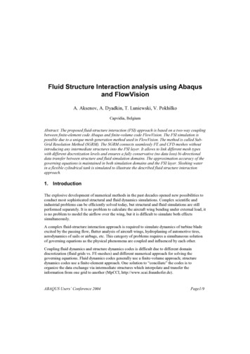
The FEM Python module enables the analyst to create automated solution sequences for anythingfrom progressive fracture to analysis sequences utilizing the full set of analysis tools as shown inFigure 1.NDE Flaw DefinitionsFEM BuilderChemical EquilibriumPerformanceCFDBurnt grainHeat TransferGrain Burn BackFEM PythonPressureCrack CombustionFracture propagationAutomated meshingPressureTemperatureStructural AnalysisFracture MechanicsStructural IntegrityDeformationStress/StrainFigure 1: Possible FEM Builder solution sequence for solid rocket motorsFEM Builder SOLVERSThe architecture of the FEM Builder software package also includes several Python classes,called solvers that encapsulate the necessary information to solve particular analyses. Forexample, a solver has been created to execute ABAQUS given a FEM Builder data filecontaining a structural model. The user provides information needed to write an ABAQUS input file, which is stored as part of the solver. The solver takes the specified model, writes anABAQUS input file, executes ABAQUS on any computer on the network, and reads theresults from the analysis back into the structural model. A similar solver has also been createdfor executing CFD models using Fluent . These two individual analysis solvers, one forstructural analysis and one for CFD analysis, are driven by a coupled FSI solver that controls thesolution sequence of a coupled solution of a fluid-structural interaction problem.Approved for public release; distribution unlimited.
Additional solvers have been developed for crack nucleation and propagation. Additional solversare currently planned to extend the analysis codes supported, as well as additional types ofcoupled analysis, which include fluid-fluid, fluid-thermal, and fluid-thermal-structural.OTHER FEM Builder FEATURESThe FEM Builder program provides most functions one might expect to find in a standard preand post processor. Standard pre-processing functions include support for: geometry creation,2D and 3D mesh generation, material property definition, and boundary condition application.FEM Builder will also import finite element modeling entities from I-DEAS Master Series andPatran . Standard post-processing functions include display of deformed geometry, contour andvector plots, as well as XY plots. Displays may be transferred for use in documentation andpresentations using the copy-to-clipboard or copy-to-bitmap options.In addition to those standard functions, FEM BuilderÓ provides a number of somewhat uniquepre- and post- processing functions. These functions include:·····Flaw insertion for 2D models. Flaws may be zero volume cracks, elliptical flaws, or generalflaws with volume; see Figure 2 - Figure 4.Result superposition.Factor of safety and margin of safety calculations for 26 different criteria as well as supportfor user defined criteria.Insertion of cracks/debonds based on continuum failure.J-Integral, Crack Closure Integral, and Crack Opening Displacement fracture mechanicscalculations.Figure 2 Crack insertionFigure 3 Elliptical voidFigure 4 General flawFEM Builder also provides a number of functions created explicitly for transferring data betweendifferent finite element models. Those functions include:··Translate, rotate, and mirror functions so that grids created in different coordinate systemscan be transformed into the same coordinate space.Interpolation of results for use as boundary conditions, e.g. interpolation of pressure from aCFD grid to a structural grid; see Figure 5.Approved for public release; distribution unlimited.
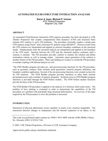
····Color boundary condition by value; see Figure 5. This function is especially useful invalidating interpolated boundary conditions.Interpolation of analysis results between models, e.g. interpolation of displacements from thestructural grid to the CFD grid in order to deform the CFD grid.Interpolation of a result for use as an initial condition, e.g. interpolation of temperature froma heat transfer grid to a structural grid.Ablation of a structural grid to match an ablated thermal grid boundary.Figure 5 Interpolated pressure boundary condition colored by valueAUTOMATED FSI ANALYSIS PROCEDUREThe automated analysis procedure uses external coupling to link CFD and structural analysis tosolve FSI problems. The approach couples a steady-state CFD analysis and a linear elasticstructural analysis. Results from each of these individual analysis codes are transferred and usedto drive the other and are iteratively solved until a solution is reached. The pressures computedin the CFD analysis are used to automatically create pressure boundary conditions on thestructural model. The displacements from the structural model are used to automatically deformthe CFD grid. This analysis procedure has been demonstrated on axisymmetric, and 3D modelsfor internal and external flow. The FEM Python module provides the backbone for the FSIsolver.A flowchart of the automated FSI analysis procedure is shown in Figure 6. The process startswith the analyst(s) preparing the CFD and structural models and setting up the FSI python script.The FSI python script initializes the automated FSI solver and iterates between the CFD andstructural analysis. The CFD analysis is performed by automatically writing an input file,executing the CFD analysis code, and reading the output file. Once the CFD analysis iscomplete, the computed pressure distribution is interpolated to specified element faces of thestructural model as pressure boundary conditions. The structural analysis is then performed bywriting an input file, executing the structural analysis code, and reading the output file.Displacement results from the structural analysis are interpolated to specified nodes of the CFDmodel. The nodes of the CFD model with displacements are then moved to their deformedpositions. The nodes that were not included in the displacement interpolation are relocated,either by re-meshing and/or smoothing, to obtain a good CFD mesh that matches the currentdeformation state of the structural model. Termination criteria control the iteration loop anddetermine when the analysis is complete. Once the FSI analysis has completed, the analystevaluates the results.Approved for public release; distribution unlimited.
AnalystAutomated FSI Analysis ProcedureModel preparationand setupFSIinitializationCFD analysiscomputes the pressureInterpolate pressure tosolid modelnoResult evaluationyesConverged?Result monitoringInterpolatedisplacement tostructural model andre-mesh/smoothStructural analysiscomputes thedisplacementsFigure 6: Basic Flowchart showing automated FSI analysis procedureOther features of the automated coupled FSI analysis include:·····Result monitoring for key nodes and/or elements during the FSI solution.Factor of Safety calculations based on user-specified failure criteriaReport generation (a Microsoft Word document) summarizing entire FSI solutionCreation of structural deformation and fluid pressure animation filesLocal or remote execution of analysis programsINTERPOLATIONOne of the enabling functions of the automated FSI coupled analysis is correct and properinterpolation of analysis results to another FE model. There are two interpolation methods usedto interpolate pressures and displacements. The first method is used in locations where the CFDgrid and the structural grid are in close proximity. For example, in pressure interpolation, thecenter of a structural element face is projected onto the CFD grid. This projection identifies theCFD element and the natural coordinates within that element of the projection point. Thepressure value at that point is interpolated from the CFD pressure result. This pressure value isthen applied as a boundary condition on the element face of the structural model. A similarApproved for public release; distribution unlimited.
operation is performed to interpolate displacements onto nodes of the CFD model in closeproximity to the structural model.The second method of interpolation is used in areas when there is a significant differencebetween the CFD model and structural model boundaries. Motor features considered critical tomodel in the structural mesh may not important in the CFD grid. Such locations may occur insolid rocket motors in the fin sections, segment joints, or stress relief flaps. This method uses anintermediate step to allow better control of the interpolation. For example, in pressureinterpolation, points of a segmented line (defined by the analyst) are interpolated onto the CFDgrid (points A and B in Figure 7). The corresponding pressures at these points are obtained, asdescribed above. The center of a structural element face is then projected onto the segmentedline and the pressure at that location is determined by linear interpolation. This pressure is thenapplied as a boundary condition on the element face of the structural model (Figure 8). Elementface centroids that project past the end points of the segmented line (points A and B) are assignedthe value at the nearest end point. Similar functions are used to interpolate displacements inthese areas onto the CFD model.AFluidFluidBSolidFigure 7: Pressure interpolation in apropellant joint/stress relief flap using asegmented line as an intermediate stepSolidFigure 8: Pressure boundary conditionsfrom pressure interpolation applied tostructural modelSAMPLE ANALYSIS – BORE CHOKINGBore choking is a possible problem in solid rocket motor designs, and has the potential ofcausing motor over-pressure and catastrophic failure. Bore choking occurs when the propellantdeforms radially inward and disrupts the flow field, causing a choked flow condition inside themotor. Bore choking is most likely to happen downstream of segment joints or radial slots. Inthis area 2D/3D CFD is necessary to accurately predict the flow field and the resulting fluidstructure interaction.The phenomenon of bore choking in a solid rocket motor is typically caused by localized areas oflow pressure. These areas of low pressure develop primarily due to flow separation downstreamof a segment joint/slot and are further enhanced by the radial flow of exhaust gas from theApproved for public release; distribution unlimited.
segment joint/slot (Figure 9). On a macro scale, a solid rocket motor is primarily onedimensional flow—the vast majority of the mass is moving in one direction. However, thelocations where bore choking is likely to occur are the areas of localized 2D/3D flow, whichrequire CFD analysis to accurately predict. The pressure difference around a downstream cornercan be significant—the CFD analysis shown in Figure 9 predicts approximately a 25.0 psi (170kPa) difference, which cannot be predicted by a one-dimensional fluid flow analysis. Thispressure difference causes the downstream corner of the propellant to deform into the flow field,enhancing the problematic flow separation. This causes greater corner deflections, and thus alower pressure. If the elastic modulus of the propellant is not stiff enough, the downstreamcorner will continue to constrict the flow, resulting in an unstable condition and bore choking.SecondaryFlow DirectionDown-streampropellant cornerLow-pressure zoneSRM propellantexhaust gasPrimary Flow DirectionFigure 9: Pressure contours of 5.0 psi (34 kPa) of flow around adown-stream corner of a segment joint/slotDESCRIPTIONThe sample bore choking analysis investigates a simple, axisymmetric solid rocket motor (SRM)design with a radial slot in the propellant2. The SRM design is shown in Figure 10 and the basicdimensions are listed in Table 1. The FSI solution is obtained for two conditions. The first2All geometry, features, and properties of this solid rocket motor and sample borechoking analysis are representative. Any resemblance to an actual solid rocket motor, real orfictitious, is purely coincidental.Approved for public release; distribution unlimited.
condition, identified as Model A, uses a propellant elastic modulus of 200 psi (1.4 MPa); thesecond condition, identified as Model B, uses a propellant elastic modulus of 500 psi (3.5 MPa).Table 1: Dimensions for solid rocket motorused in sample bore choking analysisSolid Rocket Motor DesignParametersCase LengthFigure 10: Schematic of solid rocket motorused in sample bore choking analysisCase Diameter(outside)Bore radius(slot corners)Nozzle Throat RadiusNozzle Length13.0 in(0.33 m)4.0 in(0.10 m)1.125 in(0.02858 m)0.75 in(0.019 m)6.0 in(0.15 m)SETUPThe input requirements for the FSI solver include a CFD model, a structural model, and an FSIpython script that initializes parameters needed for the FSI analysis. Additional node groups aredefined in the CFD model to indicate the nodes where displacement results are to be interpolated.An additional face groups are defined in the structural FE model to indicate the element faceswhere pressure loads are to be created.The sample axisymmetric CFD model contains a grid of the flow field, properties of the exhaustgas and propellant, boundary conditions, as well as fluid flow parameters (Figure 11).Additionally, four node groups are defined on mesh region boundaries. These nodes are used indisplacement interpolation and later deformed (Figure 12). This model is saved as a FEMBuilder data file and is specified in the FSI python script.Figure 11: CFD grid and boundaryconditionsFigure 12: Node groups for displacementinterpolationThe sample axisymmetric structural model contains a grid of the SRM, material properties, andboundary conditions (Figure 13). The nozzle was assumed not to deform, so it was not includedin the structural FE model. The model is also saved as a FEM Builder data file and is specifiedApproved for public release; distribution unlimited.
in the FSI python script. There is one additional group of element faces on the fluid-solidinterface, which is used in pressure boundary condition interpolation and application (Figure 14).Figure 13: Structural grid with restraintsFigure 14: Pressure boundary conditionsapplied to element face group# Example 11 - Coupled Fluid-Solid Analysis#Import necessary modulesfrom CExecuteFluent import *from CExecuteAbaqus import *from CSolveCoupledFSISteady import *#Assign class valuesLESS CSolveCoupledFSISteady()Solid CExecuteAbaqus()Fluid tandardPostFunctions()#Initialize Solid member nits('In, ions()Solid.AddFoSCriteria('Energy Density')#Initialize Fluid member nits('In, F')Fluid.SetMaxTime(1.0)#Fluent etLimits(LimitMinT 20.0, LimitMaxT 10000.0, LimitMinP 2.0, LimitMaxP 3000.0,LimitMaxViscRatio alize LESS member essure')LESS.SetBCLoading([0.50, 'Pressure','Max',5.0e-3)# Define pressure interpolation operationsLESS.AddPressureBCInterpolation('Face', 'FluidInterface', MaxProject .05)#Define displacement interpolation , 'SolidInterface', MaxProject 0.05)LESS.AddDisplacementInterpolation('Project', 'ProjectDisp', Nodes al', 'FwdRadialDisp', Nodes [857])LESS.AddDisplacementInterpolation('Radial', 'AftRadialDisp', Nodes SS.CloseAllViews()Figure 15: FSI python script for sample bore choking analysisApproved for public release; distribution unlimited.
The FSI python script contains the file names of the CFD and structural models, informationabout writing input files, executing the CFD and structural analysis, and other data required toperform a coupled FSI analysis. Figure 15 is a sample FSI python script for this bore chokinganalysis. It is included only to illustrate the simple form of the input.EXECUTIONThis sample bore choking analysis used Fluent for the CFD analysis, and ABAQUS for thestructural analysis. Each FSI analysis took approximately two and a half minutes on a PC withWindows XP with a 2.8 GHz processor with 512 GB of RAM. Obviously larger and morecomplex models will take longer to run. The short execution time illustrates the quick analysistime made possible with the automated FSI analysis procedure. The procedure can be set up toexecute the CFD and structural analysis codes anywhere on the LAN.RESULTSThe sample bore choking analysis for this solid rocket motor showed that bore choking occurredwhen the elastic propellant modulus was 200 psi, but not when the elastic modulus was 500 psi.Table 2 compares several key output results.Table 2: Select Results from sample bore choking analysisResultNumber of iterationsHead end pressure at final stepMaximum radial displacement atfinal stepMaximum axial displacement atfinal stepBore chokedModel B500 psi(3.4 MPa)Model A200 psi(1.4 MPa)5747.55 psi(5.154 MPa)-1.185 in(-3.009 cm)1.724 in(4.379 cm)Yes7622.83 psi(4.294 MPa)-0.058 in(-0.147 cm)0.114 in (0.289 cm)NoThe analysis of Model A indicates continued inward deflection of the downstream slot corner,which increases in magnitude with each subsequent FSI iteration, as shown in Figure 17. Thesixth CFD solution for Model A failed because the deformations applied from the previousstructural analysis caused the downstream slot corner to deform past the centerline (Figure 16),indicating a choked flow condition.Approved for public release; distribution unlimited.
CenterlineFigure 16: Solid model with E 200 psishowing initial and final propellantdeformationsFigure 17: Detail of slot with E 200 psishowing intermediate propellantdeformationsThe analysis of Model B did not exhibit the instability of Model A; compare Figure 17 andFigure 19. The FSI solution iterated to a converged solution in seven steps. The inwarddeflection of the downstream slot corner did not become unstable, as it did in Model A. Both thepressure and the deformations converged to a stable solution, as shown in the plots of Figure 20and Figure 21.CenterlineFigure 19: Detail of slot with E 500 psishowing intermediate propellantdeformationsFigure 18: Solid model with E 500 psishowing initial and final propellantdeformationsHead End Pressure8002.0Displacement (in)Pressure (psi)750700650600M odel A550M odel BDownstream Slot CornerDisplacements1.00.0M odel A dR-1.0M odel A dUM odel B dRM odel B dU-2.050012345617Figure 20: Plot of head end pressure forModel A and Model B234567IterationIterationFigure 21: Plot of downstream slot cornerdisplacement for Model A and Model BApproved for public release; distribution unlimited.
Additional FSI solutions were performed for this motor design for several different values of thepropellant elastic modulus between 200 psi (1.4 MPa) and 500 psi (3.4 MPa). The results ofthese analyses indicate that the elastic modulus of the propellant must be 350 psi or above toprevent motor failure by bore choking. The results from these analyses are summaries in Table 3and Figure 22.Motor StabilityTable 3: Motor Stability listed for values ofelastic modulus and number of iterationsNumber leUnstableUnstableUnstableUnstableNumber of 25St able20Unstable151050100200300400500600Elastic Modulus (psi)Figure 22: Plot of number of iterations vs.elastic modulusFUTURE DEVELOPMENTThe future development plans for the FEM Builder software package includes the addition ofFEM Builder solver for thermal analysis to the coupled FSI solution. Besides adding a thermalsolver, a 2D thermal ablation finite element code will be developed and used in this coupledanalysis environment to model the thermal ablation of a SRM nozzles.CONCLUSIONSThe automated FSI analysis procedure developed at ATK Thiokol Propulsion externally couplesCFD and structural analyses using Fluent and ABAQUS , respectively. The approach isstraightforward and fairly simple to use. The automated feature of the FSI analysis proceduremakes this method very fast and economical to use, especially when compared to doing the sameanalysis manually. The automated FSI procedure has application in analysis, as well as design.REFERENCES1. Python programming language at www.python.orgApproved for public release; distribution unlimited.
NOMENCLATURE, ACRONYMS, ABBREVIATIONSCFDComputational Fluid DynamicsFEFinite ElementFEM Finite Element ModelFSIFluid Structure InteractionLAN Local Area NetworkSRM Solid Rocket MotorRSRM Reusable Solid Rocket MotorApproved for public release; distribution unlimited.
CFD analysis using Fluent and a structural FE analysis using ABAQUS . Pressure results from the CFD solution are interpolated and applied as pressure boundary conditions on the structural model. Displacements from the structural analysis are interpolated and applied to the boundary of the CFD mesh.