Transcription
Visualization of Large Networks with Min-cutPlots, A-plots and R-MAT , Deepayan Chakrabarti a Christos Faloutsos b Yiping Zhan ca ResearchScientist, Yahoo! Research, 701 1st Ave, Sunnyvale, CA 94089.b Professor,c WorkSchool of Computer Science, CMU, Pittsburgh, PA 15213.done while a Ph.D. candidate in the Dept. of Biological Sciences and Schoolof Computer Science, CMU, Pittsburgh, PA 15213.AbstractWhat does a ‘normal’ computer (or social) network look like? How can we spot‘abnormal’ sub-networks in the Internet, or web graph? The answer to such questionsis vital for outlier detection (terrorist networks, or illegal money-laundering rings),forecasting, and simulations (“how will a computer virus spread?”).The heart of the problem is finding the properties of real graphs that seem topersist over multiple disciplines. We list such patterns and “laws”, including the“min-cut plots” discovered by us. This is the first part of our NetMine package: givenany large graph, it provides visual feedback about these patterns; any significantdeviations from the expected patterns can thus be immediately flagged by the useras abnormalities in the graph. The second part of NetMine is the A-plots toolfor visualizing the adjacency matrix of the graph in innovative new ways, againto find outliers. Third, NetMine contains the R-MAT (Recursive MATrix) graphgenerator, which can successfully model many of the patterns found in real-worldgraphs and quickly generate realistic graphs, capturing the essence of each graph inonly a few parameters. We present results on multiple, large real graphs, where weshow the effectiveness of our approach.Key words: Min-cut plots, A-plots, R-MAT, abnormal subgraphs, graph generator Previous versions of this material were presented in SIAM Data Mining 2004 andin the SIAM DM 2004 Workshop on Link Analysis, Counter-terrorism and Privacy. This material is based upon work supported by the National Science Foundationunder Grants No. IIS-0083148, IIS-0113089, IIS-0209107 IIS-0205224 INT-0318547SENSOR-0329549 EF-0331657IIS-0326322 CNS-0433540 by the Pennsylvania Infrastructure Technology Alliance (PITA) Grant No. 22-901-0001. Additional funding was provided by donations from Intel, and by a gift from Northrop-GrummanPreprint submitted to Elsevier Science26 March 2006
1IntroductionGraphs and networks have attracted significant interest recently, due to theirability to model many distinct real-world datasets under one intuitive framework. For example, the World Wide Web of webpages connected by hyperlinks,the Internet of computers connected by routers, social networks of individuals,protein interaction networks, and many other datasets can be easily expressedas a graph of nodes (webpages, computers, individuals, etc.) connected byedges (hyperlinks, routing links, etc.) The question we must ask is: How canwe visualize the information contained in such large graphs efficiently?Laying out the graph on a computer screen quickly becomes a hard problem as the graph size grows to millions (or even billions) of nodes of edges(such as the WWW graph). One solution is to look for patterns or motifs thatappear in most real-world graphs, and indeed, many surprising regularitiesand “laws” have recently been discovered. The World Wide Web, the Internet topology and Peer-to-Peer networks follows surprising power-laws (Broderet al., 2000; Faloutsos et al., 1999; Barabási, 2002), exhibit strange “bow-tie”or “jellyfish” structures (Broder et al., 2000; Tauro et al., 2001), while stillhaving a small diameter (Albert and Barabási, 2002). Finding patterns, lawsand regularities in large real networks has numerous applications, from criminology and law enforcement (Chen et al., 2003) to analyzing virus propagationpatterns (Pastor-Satorras and Vespignani, 2001) and understanding networksof regulatory genes and interacting proteins (Barabási, 2002) and so on. Amethod for visualizing common patterns can immediately tell the user howthe given graphs matches “expectations,” and whether there are any abnormalities that merit further attention.To find better patterns (and, concurrently, better anomaly detection algorithms), we need to model real-world graphs well. In other words, we candevelop a good graph generator, which can create synthetic yet “realistic”graphs. Then, given any graph as input, we can check to see if the generatorcan build a “similar” graph under any set of parameters. If not, then it mightrepresent an anomaly in the input graph, such as a misconfigured router inthe Internet graph.Which patterns should we be looking for? How can we spot suspicious/erroneoussubgraphs quickly? These are the questions that our NetMine system focuseson. The main contributions of this paper are that it proposes the “min-cut plots”, an interesting pattern to check for whileCorporation. Any opinions, findings, and conclusions or recommendations expressedin this material are those of the author(s) and do not necessarily reflect the viewsof the National Science Foundation, or other funding parties.2
analyzing a graphit proposes the “A-plots” as a tool for quickly finding suspicious subgraphs/nodesit scales very well with size of the graph for all its tasks, and thus is able toquickly handle graphs of hundreds of thousands of nodesit shows how to interpret these plots, and how we found surprising patternsand outliers on real graphsfinally, it describes a recent, promising graph generator, “R-MAT”, so thatthe user could generate similar, synthetic graphs.The rest of this paper is organized as follows: Section 2 surveys the existinggraph laws and generators. Section 3 presents our proposed methods and algorithms for mining large graphs. Section 4 gives the experimental results. Weconclude in Section 5.2Background and Related WorkA graph G (V, E), is a set V of N nodes, and a set E of E edges between them.The adjacency matrix A of graph G is an N N matrix, with entry a(i, j) 1if the edge (i, j) exists, and 0 otherwise. The edges may be undirected (likethe network of Internet routers and their physical links) or directed (like thenetwork of who-trusts-whom in the epinions.com database (Richardson andDomingos, 2002)). Bipartite graphs have edges between two sets of nodes,like, for example, the graph of the movie-actor database (www.imdb.com). Wesplit the discussion of related work into two parts: graph patterns, and graphgenerators.2.1 Patterns and “Laws”Skewed distributions, and power laws of the form y xa , appear very often.Power-laws have been observed for the degree distributions of the Internet,the WWW and the citation graph, the distribution of “bipartite cores” ( communities), the eigenvalues of the adjacency matrix and others (Faloutsoset al., 1999; Kleinberg et al., 1999; Albert and Barabási, 2002). Recently, Pennock et al. (Pennock et al., 2002) observed deviations from power-laws for theWeb graph, which are well-modeled by the truncated, discretized lognormal(“DGX”) distribution of Bi et al. (Bi et al., 2001). Graphs also exhibit a strong“community” effect (Gibson et al., 1998; Kumar et al., 1999). Most real graphslike the Web and the Internet have surprisingly small diameters (Albert andBarabási, 2002; Tauro et al., 2001).Apart from these, there are many othermeasures such as clustering coefficient, expansion, resilience, prestige, influence, stress and so on (Chakrabarti, 2002; Gkantsidis et al., 2003; Tangmu3
narunkit et al., 2001; Palmer et al., 2002). Broder et al. (Broder et al., 2000)show that the WWW has a “bow-tie” structure, while Tauro et al. (Tauroet al., 2001) find that the Internet topology is organized as a set of concentriccircles around a small core, like a “Jellyfish”.2.2 Graph GeneratorsThe earliest graph generating model is by Erdős and Rényi. However it provably violates the power laws above. Recent graph generators can be groupedin two classes: degree based and procedural. Given a degree distribution (typically following a power-law), the degree-based ones try to find a graph thatmatches it (Albert and Barabási, 2002; Newman, 2003), but without giving anyinsights about the graph or trying to match other criteria (like small diameter,eigenvalues etc.). On the other hand, procedural generators (like our proposedR-MAT method) try to find simple mechanisms to generate graphs that matcha property of the real graphs and, typically, the power law degree distribution.The typical representative here is the Barabasi-Albert (BA) method with the“preferential attachment” idea: keep adding nodes; new nodes prefer to connect to existing nodes with high degrees. Many modifications and alternativesto the basic idea have been proposed; some generators also include the geometrical layout of nodes in their models (Albert and Barabási, 2000, 2002;Newman, 2003; Pennock et al., 2002; Bu and Towsley, 2002). The BRITEgenerator (Medina et al., 2000) uses components from several of the abovemodels.In general, all of the above generators fail to meet one or more of the followinggoals: (a) the generator should be procedural (b) it should be able to generateall types of graphs (directed/undirected, bipartite, weighted) (c) it shouldmatch both power-law degree distributions and the “unimodal” distributionsobserved by Pennock et al. (Pennock et al., 2002) (d) it should satisfy morecriteria (like diameter, eigenvalue plots), in addition to the degree distribution.A related field is that of relational learning (Dzeroski and Lavrac, 2001); however, this focuses on finding structure at a more local level while our workfocuses on the global level. Other topics of interest involving graphs includegraph partitioning,frequent subgraph discovery,finding cycles in graphs,andmany others. These address interesting problems, and we are investigatingtheir use in our work.4
Min t/edges)-4N 0.5-5-6-7-8O(N(a) A grid and its min-cut-4-5-6-7-9-10-10)Slope )1618200246810 12log(edges)14161820(b) 2D grid min-cut plot (c) Averaged min-cut plotFig. 1. Plot (a) shows a portion of a regular 400x400 2D grid, and a possible min-cut.Plot (b) shows the full min-cut plot, and plot (c) shows the averaged plot. If thenumber of nodes is N , the length of each side is N . Then the size of the min-cutis O( N ), which leads to a slope of 0.5, which is exactly what we observe.3Proposed MethodThe contributions of NetMine are threefold: (1) we present the “min-cutplots”, a new pattern for comparing a synthetically-generated graph to a realone; this is in addition to the list of patterns described in Section 2 above,(2) we present a novel tool called A-plots for interactive inspection of graphsand for finding erroneous/outlier nodes and subgraphs, and (3) we present theR-MAT graph generator, which can match almost all these patterns. Each ofthese provides us with a tool to visually probe the graph dataset; they letus infer, at a glance, some interesting properties of the graph while, at thesame time, highlighting possible anomalies. In this section, we describe eachof these parts; the observations we can make from visualizing them are betterexplained via experiments, described later in section 4.3.1 “Min-cut plots”:Several criteria have been previously proposed to compare a synthetic graph toa real-world graph. These include degree distributions, hop-plots, scree-plotsand others. NetMine includes all these, and adds “min-cut plots”.A min-cut of a graph G (V, E) is a partition of the set of vertices V intotwo sets V1 and V V 1 such that both partitions are of approximately thesame size, and the number of edges crossing partition boundaries is minimized.The number of such edges in the min-cut is called the min-cut size. Min-cutsizes of various classes of graphs has been studied extensively, and are knownto have important effects on other properties of the graphs (Rosenberg andHeath, 2001). For example, Figure 1(a) shows a regular 2D grid graph, andone possible min-cut of the graph. We see that if the number of nodes is N,then the size of the min-cut (in this case) is O( N).5
The min-cut plot is built as follows: given a graph, its min-cut is found, andthe set of edges crossing partition boundaries deleted. This divides the graphinto two disjoint graphs; the min-cut algorithm is then applied recursively toeach of these sub-graphs. This continues till the size of the graph reaches asmall value (set to 20 in our case). Each application of the min-cut algorithmbecomes a point in the min-cut plot. The graphs are drawn on a log-log scale.The x-axis is the number of edges in a given graph. The y-axis is the fractionof that graph’s edges that were included in the edge-cut for that graph’sseparator.Figure 1(b) shows the min-cut plot for the 2D grid graph. In plot (c), thevalue on the y-axis is averagedover all points having the same x-coordinate. The min-cut size is O( N ), so this plot should have a slope of 0.5, whichis exactly what we observe. In section 4, we will see how the min-cut plots ofreal-world graphs look like, and how their similarities with figure 1 allow usto characterize them.3.2 A-plots:A simple way to find suspicious nodes/subgraphs in a large graph could bevery useful in a variety of situations. However, the obvious approach of tryingto visualize the graph does not work very well: visualization of large graphs isnotoriously tough and time consuming, and is a research topic in its own right.Our next tool, called A-plots, is another way to visually hunt for anomalies.It consists of three types of plots for undirected graphs: (1) the plot of theadjacency matrix with nodes sorted in decreasing order by their network values(RV -RV plot, for Rank of network Value), (2) the plot of the degree of anode verses its rank of network value (D-RV plot, for Degree verses Rank ofnetwork Value), and (3) the plot of the adjacency matrix with nodes sorted indecreasing order by their degrees (RD-RD plot, for Rank of Degree). Together,these plots often reveal interesting patterns and properties of the graph.Consider, for example, the D-RV plot for, say, the Internet router graph. Ingeneral, we expect nodes with high degree to be near the core of the graph(the Internet “backbone”), and thus also have high network value. Thus, beforeseeing the D-RV plot, we might expect it to decay smoothly, with low degreebeing correlated with low rank in network value. However, as we shall inSection 4, there are sudden spikes in this plot, which we can immediatelypick out visually as outliers. Thus, visual inspection of the D-RV plot revealsanomalies which might have gone unnoticed otherwise. The reasons behindthis particular anomaly will be discussed later in Section 4.6
3.3 The R-MAT generator:A good graph generator, with a proper choice of parameters, should be ableto match a given real-world graph; the absence of a good match may indicateabnormalities in the given graph. Several previous graph generators have beendescribed in Section 2, but they all fail in one aspect or another. The goals agraph generator should achieve are that the generated graph should: (g1) match the degree distributions (power laws or not) (g2) exhibit a “community” structure (g3) have a small diameter, and match other criteria.A good generator, matching these patterns, can be useful for many applications: Detection of abnormal subgraphs/edges/nodes: Abnormalities should deviatefrom the “normal” patterns, so a good graph generator will not be able tomatch an abnormal graph very well. Thus, given an input graph, we cancheck for anomalies using a three-step process: (1) find the best matchingparameter set for our graph generator, (2) generate a synthetic graph usingthese parameters, and (3) visually compare the patterns of the input graphagainst the generated graph. Absence of a fit may point to anomalies. Simulation studies: Algorithms meant for large real-world graphs can betested on synthetic graphs which “look like” the original graphs. This isparticularly useful if collecting the real data is hard or costly. Realism of samples: Most graph algorithms are super-linear on the nodecount, and thus prohibitive for large graphs. We might want to build asmall sample graph that is “similar” to a given large graph. In other words,this smaller graph needs to match the “patterns” of the large graph to berealistic. Extrapolation of data: Given a real, evolving graph, we expect it to have x%more nodes next year; how will it then look like, assuming that our “laws”are still obeyed? For example, in order to test the next-generation Internetprotocol, we would like to simulate it on a graph that is “similar” to whatthe Internet will look like a few years into the future.In the following, we will describe our R-MAT graph generator, show that itmatches goals g1-g3, and develop a parameter-fitting method for it.3.3.0.1 Main Idea: We provide a method which fits both unimodal andpower-law graphs using very few parameters. Our method, called RecursiveMATrix, or R-MAT for short, generates the graph by operating on its adjacency matrix in a recursive manner. Recursive generators have been proposed7
ToNodesFromacabdbcNodescddFig. 2. The R-MAT modelin passing before (Palmer and Steffan, 2000), but the emphasis was on networkissues.3.3.0.2 Fast Algorithm to generate Directed Graphs: Recall that theadjacency matrix A of a graph of N nodes is an N N matrix, with entrya(i, j) 1 if the edge (i, j) exists, and 0 otherwise. The basic idea behind RMAT is to recursively subdivide the adjacency matrix into four equal-sizedpartitions, and distribute edges within these partitions with a unequal probabilities: starting off with an empty adjacency matrix, we “drop” edges intothe matrix one at a time. Each edge chooses one of the four partitions withprobabilities a, b, c, d respectively (see Figure 2). Of course, a b c d 1.The chosen partition is again subdivided into four smaller partitions, and theprocedure is repeated until we reach a simple cell ( 1 1 partition). This isthe cell of the adjacency matrix occupied by the edge. The number of nodes inthe R-MAT graph is set to 2n ; typically n ⌈log2 N⌉. There is a subtle pointhere: we may have duplicate edges (ie., edges which fall into the same cell inthe adjacency matrix), but we only keep one of them. To smooth out fluctuations in the degree distributions, we add some noise to the (a, b, c, d) values ateach stage of the recursion and then renormalize (so that a b c d 1).Table 1 shows the symbols used in the paper.3.3.0.3 Discussion: Meeting the Goals: Intuitively, our technique is generating “communities” in the graph. Typically, a b, a c, a d. The partitions a and d represent separate groups of nodes which correspondto communities (say, soccer and automobile enthusiasts). The partitions b and c are the cross-links between these two groups; edgesthere would denote friends with separate interests. The recursive nature of the partitions means that we automatically getsub-communities within existing communities (say, motorcycle and car enthusiasts within the automobile group).8
SymbolMeaningNNumber of nodes in the real graph2nNumber of nodes in the R-MAT graphENumber of edges in the real graph, andin the R-MAT generated graph afterduplicate elimination(a, b, c, d)Probabilities of an edge falling into partitionsin the R-MAT model. a b c d 1.Table 1Table of symbols.The third bullet results in “communities within communities” (goal g2). Theskew in the distribution of edges between the partitions (a d) leads tolognormals and the DGX distribution (goal g1). We shall show experimentallythat R-MAT also generates graphs with small diameter and matching othercriteria as well (goal g3).3.3.0.4 Parameter fitting with AutoMAT-fast: The R-MAT model canbe considered as a binomial cascade in two dimensions. We can calculate theexpected number of nodes ck with out-degree k:!! niE kik hn h n iE Xp (1 p)i 1 pn i (1 p)ick k i 0 iwhere 2n is the number of nodes in the R-MAT graph and p a b. Fittingthis to the observed outdegree distribution gives us the estimated values forp a b (and similarly q a c for the indegree distribution). Conjecturingthat the a : b and a : c ratios are approximately 75 : 25 (as seen in many realworld scenarios), we can calculate the parameters (a, b, c, d).3.3.0.5 Extending R-MAT to Undirected Graphs: An undirected graphmust have a symmetric adjacency matrix. We achieve this by generating a directed graph with b c and then using a “clip-and-flip” on the resultingadjacency matrix. This involves throwing away the half of matrix above themain diagonal and copying the lower half to it. The effect of this is twofold:first, since b c, the number of edges in the final undirected matrix is approximately equal to that in the directed graph; and second, this techniqueguarantees that the resulting matrix will be symmetric, and hence the corresponding graph will be undirected.9
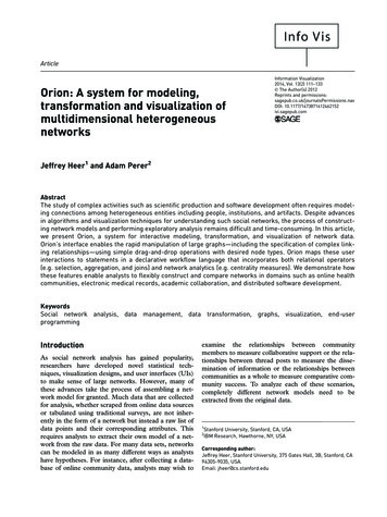
3.3.0.6 Extending R-MAT to Bipartite Graphs: For a bipartite graph,the length and height may be different, and the adjacency matrix will be arectangle instead of a square. Here too, we set the length and width to bepowers of 2, denoted by 2n1 and 2n2 . While dropping edges, we might form apartition with a length(height) of 1; in such a case, further partitions are justtop-bottom(left-right) with the appropriate probabilities.4ExperimentsThe questions we wish to answer are: [Q1] How do the min-cut plots look for real-world graphs? Does R-MATmatch them? What can the min-cut plot tell us about the graph? [Q2] How can A-plots be used for analyzing large graphs? [Q3] How does R-MAT compare with existing generators for undirectedgraphs? [Q4] How does R-MAT compare with existing generators for directed graphs? [Q5] How does R-MAT compare with existing generators for bipartite graphs?The datasets we use for our experiments are: Epinions: A directed graph of who-trusts-whom from epinions.com (Richardson and Domingos, 2002): N 75, 879; E 508, 960. Epinions-U: An undirected version of the Epinions graph: N 75, 879; E 811, 602. Clickstream: A bipartite graph of Internet users’ browsing behavior (Montgomery and Faloutsos, 2001). An edge (u, p) denotes that user u accessedpage p. It has 23, 396 users, 199, 308 pages and 952, 580 edges. Lucent is an undirected graph of network routers, obtained from www.isi.edu/scan/mercator/maps.html. N 112, 969; E 181, 639. Router is a larger graph (the SCAN Lucent map) from the same URL,which subsumes the Lucent graph. N 284, 805; E 898, 492. Google is a graph of webpage connectivity from the Google (Google Programming Contest, 2002) programming contest. N 916, 428; E 5, 105, 039.4.1 [Q1] Min-cut Plots:What do the min-cut plots for real-world graphs look like? Are they like mincut plots for random graphs, or are they completely different? Figure 3 showsmin-cut sizes of some real-world graphs. For each graph, we used the Metisgraph partitioning library (Karypis and Kumar, 1995) to generate a separator,10
log(mincut/edges)-4-6-8-10-1246810 12 14 16 18 20 22log(edges)(a) “Google” min-cut plot0-280-210 12 es)(d) “Google” averaged10 12 6-1-4-4(b) “Lucent” min-cut plot (c) “Clickstream” min-cut 0log(edges)12141618(e) “Lucent” averaged0246810 12log(edges)141618(f) “Clickstream” averagedFig. 3. These are the min-cut plots for several datasets. We plot the ratio of mincut-size to edges versus number of edges on a log-log scale. The first row shows theactual plots; in the second row, the cutsize-to-edge ratio is averaged over all pointswith the same number of edges.as described by Blandford, Blelloch, and Kash (Blandford et al., 2003).For random graphs, we expect about half the edges to be included in the cut.Hence, the min-cut plot of a random graph would be a straight horizontalline with a y-coordinate of about log(0.5) 1. A very separable graph (forexample, a line graph) might have only one edge in the cut; such a graph withN edges would have a y-coordinate of log(1/N) log(N), and its min-cutplot would thus be on the line y x.As we can see from Figure 3, the plots for real-world graphs do not matcheither of these situations, meaning that real-world graphs are quite far fromeither random graphs or simple line graphs. Indeed, it appears as if the graphlooks like a grid when the number of edges is low (as in figure 1), but with adistinguishing “lip” when the number of edges is very high.Observation 1 (Noise) We see that real-world graphs seem to have a lot of“noise” in their min-cut plots, as shown by the first row of Figure 3.Observation 2 (“Lip”) The ratio of min-cut size to number of edges decreases with increasing edges, except for graphs with large number of edges,where we observe a “lip” in the min-cut plot.Thus, the min-cut plot seems to have a linear slope over a wide range of thex-axis, but with a (as yet unexplained) “lip” at the end. Now, given any real1120
-1Real Epinions dataR-MAT generated t/edges)log(mincut/edges)0-1-2-3-4-5-646810 12 14 16 18 20log(edges)(a) “Epinions” 1618(b) R-MAT min-cuts-4.502468 10 12 14 16 18 20log(edges)(c) Averaged min-cutsFig. 4. Here, we compare min-cut plots for the Epinions dataset and a datasetgenerated by R-MAT, using properly chosen parameters (in this case, a 0.5, b 0.2,c 0.2, d 0.1) We see from plot (c) that the shapes of the min-cut plots are similar.world graph, we can visualize its min-cut plot, and any significant deviationsfrom this general pattern might be due to anomalies in the graph.The min-cut plot contains important information about the graph (Rosenbergand Heath, 2001). Hence, any synthetically generated graph meant to simulatea real-world graph should match the min-cut plot of the real-world graph. InFigure 4, we compare the mincut-plots for the Epinions graph with a graphgenerated R-MAT. As can be seen, the basic shape of the plot is the same inboth cases, though the R-MAT plot appears to be shifted slightly from theoriginal.Observation 3 The graphs generated by R-MAT appear to match the basicshape of the min-cut plot for several real-world graphs.Summary of min-cut plots: Given an input graph, the min-cut plot is a usefulvisual tool which helps us understand its structure. Most real-world graphsexhibit high noise, but on average, they look like a grid (in some dimension)for low values on the x-axis, and a “lip” for high values. Significant deviationsfrom this pattern would indicate the presence of outliers at some scale in thegraph.4.2 [Q2] A-plots:Figures 5 and 6 show A-plots for the Router dataset. Figure 5 shows theRV -RV and RD-RD plots, and Figure 6 shows the D-RV plot under differentscalings. We can make the following observations:Observation 4 (“Water-Drop”) The RV -RV plot has a clean and smoothoval-shaped boundary for the edges in the graph.12
(a) RV -RV plot(b) Estimated boundaries(c) RD-RD plotRank of Network ValueStripesRank of Network ValueDegree 1nodesDegree 2nodesRank of Network ValueRank of 00000011111111111111111111111111111111Rank of Network 1111100000111110000011111000001111100000111
Visualization of Large Networks with Min-cut Plots, A-plots and R-MAT , Deepayan Chakrabartia Christos Faloutsosb Yiping Zhanc aResearch Scientist, Yahoo!Research, 701 1st Ave, Sunnyvale, CA 94089. bProfessor, School of Computer Science, CMU, Pittsburgh, PA 15213. cWork done while a Ph.D. candidate in the Dept. of Biological Sciences and School of Computer Science, CMU, Pittsburgh, PA .