WIXLIB

In Section 7, we discuss the performance of statistical arbitrage in 2007,and particularly around the inception of the liquidity crisis of August 2007. Wecompare the performances of the mean-reversion strategies with the ones studiedin the recent work of Khandani and Lo (2007). Conclusions are presented inSection 8.2A quantitative view of risk-factors and marketneutralityWe divide the world schematically into “indexers’ and “market-neutral agents”.Indexers seek exposure to the entire market or to specific industry sectors. Theirgoal is generally to be long the market or sector with appropriate weightings ineach stock. Market-neutral agents seek returns which are uncorrelated with themarket.NLet us denote by {Ri }i 1 the returns of the different stocks in the tradinguniverse over an arbitrary one-day period (from close to close). Let F representthe return of the “market portfolio” over the same period, (e.g. the return ona capitalization-weighted index, such as the S&P 500). We can write, for eachstock in the universe,Ri βi F R̃i ,(4)which is a simple regression model decomposing stock returns into a systematiccomponent βi F and an (uncorrelated) idiosyncratic component R̃i . Alternatively, we consider multi-factor models of the formRi mXβij Fj R̃i .(5)j 1Here there are m factors, which can be thought of as the returns of “benchmark”portfolios representing systematic factors. A trading portfolio is said to beNmarket-neutral if the dollar amounts {Qi }i 1 invested in each of the stocks aresuch thatβj NXβij Qi 0,j 1, 2, ., m.(6)i 1The coefficients β j correspond to the portfolio betas, or projections of the portfolio returns on the different factors. A market-neutral portfolio has vanishingportfolio betas; it is uncorrelated with the market portfolio or factors that drivethe market returns. It follows that the portfolio returns satisfy5

NXQi Ri i 1NX mNXX Qiβij Fj Qi R̃ii 1 mXj 1"j 1 NXNXi 1#βij Qi Fj i 1NXQi R̃ii 1Qi R̃i(7)i 1Thus, a market-neutral portfolio is affected only by idiosyncratic returns. Weshall see below that, in G8 economies, stock returns are explained by approximately m 15 factors (or between 10 and 20 factors), and that the the systematic component of stock returns explains approximately 50% of the variance (seePlerou et al. (2002) and Laloux et al. (2000)). The question is how to define“factors”.2.1The PCA approach: can you hear the shape of themarket?A first approach for extracting factors from data is to use Principal ComponentsAnalysis (Jolliffe (2002)). This approach uses historical share-price data on across-section of N stocks going back, say, M days in history. For simplicityof exposition, the cross-section is assumed to be identical to the investmentuniverse, although this need not be the case in practice.3 Let us represent thestocks return data, on any given date t0 , going back M 1 days as a matrixRik Si(t0 (k 1) t) Si(t0 k t), k 1, ., M, i 1, ., N,Si(t0 k t)where Sit is the price of stock i at time t adjusted for dividends and t 1/252.Since some stocks are more volatile than others, it is convenient to work withstandardized returns,Yik whereRi Rik RiσiM1 XRikMk 1andMσ 2i 1 X(Rik Ri )2M 1k 13 For instance, the analysis can be restricted to the members of the S&P500 index in theUS, the Eurostoxx 350 in Europe, etc.6

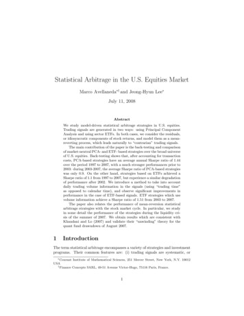
The empirical correlation matrix of the data is defined byMρij 1 XYik Yjk ,M 1(8)k 1which is symmetric and non-negative definite. Notice that, for any index i, wehaveρii1 M 1MXk 1MP2(Yik )1 k 1 M 1(Rik Ri )2σ 2i 1.The dimensions of ρ are typically 500 by 500, or 1000 by 1000, but the datais small relative to the number of parameters that need to be estimated. Infact, if we consider daily returns, we are faced with the problem that very longestimation windows M N don’t make sense because they take into accountthe distant past which is economically irrelevant. On the other hand, if we justconsider the behavior of the market over the past year, for example, then we arefaced with the fact that there are considerably more entries in the correlationmatrix than data points.The commonly used solution to extract meaningful information from thedata is Principal Components Analysis.4 We consider the eigenvectors andeigenvalues of the empirical correlation matrix and rank the eigenvalues in decreasing order:N λ1 λ2 λ3 . λN 0.We denote the corresponding eigenvectors by (j)(j)v (j) v1 , ., vN, j 1, ., N.A cursory analysis of the eigenvalues shows that the spectrum contains a fewlarge eigenvalues which are detached from the rest of the spectrum (see Figure1). We can also look at the density of statesD(x, y) {#of eigenvalues between x and y}N(see Figure 2). For intervals (x, y) near zero, the function D(x, y) correspondsto the “bulk spectrum” or “noise spectrum” of the correlation matrix. Theeigenvalues at the top of the spectrum which are isolated from the bulk spectrumare obviously significant. The problem that is immediately evident by lookingat Figures 1 and 2 is that there are less “detached” eigenvalues than industrysectors. Therefore, we expect that the boundary between “significant” and“noise” eigenvalues to be somewhat blurred and to correspond to be at the4 We refer the reader to Laloux et al. (2000), and Plerou et al. (2002) who studied thecorrelation matrix of the top 500 stocks in the US in this context.7

Figure 1: Eigenvalues of the correlation matrix of market returns computedon May 1 2007 estimated using a 1-year window (measured as percentage ofexplained variance)Figure 2: The density of states for May 1-2007 estimated using a year window8

edge of the “bulk spectrum”. This leads to two possibilities: (a) we take intoaccount a fixed number of eigenvalues to extract the factors (assuming a numberclose to the number of industry sectors) or (b) we take a variable number ofeigenvectors, depending on the estimation date, in such a way that a sum of theretained eigenvalues exceeds a given percentage of the trace of the correlationmatrix. The latter condition is equivalent to saying that the truncation explainsa given percentage of the total variance of the system.Let λ1 , ., λm , m N be the significant eigenvalues in the above sense. Foreach index j, we consider a the corresponding “eigenportfolio”, which is suchthat the respective amounts invested in each of the stocks is defined as(j)(j)Qi vi.σiThe eigenportfolio returns are thereforeFjk N(j)Xvii 1σiRikj 1, 2, ., m.(9)It is easy for the reader to check that the eigenportfolio returns are uncorrelatedin the sense that the empirical correlation of Fj and Fj 0 vanishes for j 6 j 0 . Thefactors in the PCA approach are the eigenportofolio returns.Figure 3: Comparative evolution of the principal eigenportfolio and thecapitalization-weighted portfolio from May 2006 to April 2007. Both portfolios exhibit similar behavior.Each stock return in the investment universe can be decomposed into itsprojection on the m factors and a residual, as in equation (4). Thus, the PCA9

approach delivers a natural set of risk-factors that can be used to decompose ourreturns. It is not difficult to verify that this approach corresponds to modelingthe correlation matrix of stock returns as a sum of a rank-m matrix corresponding to the significant spectrum and a diagonal matrix of full rank,ρij mX(k) (k)λk vi vj 2ii δij ,k 0where δij is the Kronecker delta and 2ii is given by 2ii 1 mX(k) (k)λk vi vik 0so that ρii 1. This means that we keep only the significant eigenvalues/eigenvectorsof the correlation matrix and add a diagonal “noise” matrix for the purposes ofconserving the total variance of the system.2.2Interpretation of the eigenvectors/eigenportfoliosAs pointed out by several authors (see for instance, Laloux et al.(2000)), thedominant eigenvector is associated with the “market portfolio”, in the sense(1)that all the coefficients vi , i 1, 2., N are positive. Thus, the eigenport(1)v(1)folio has positive weights Qi σi i . We notice that these weights are inversely proportional to the stock’s volatility. This weighting is consistent withthe capitalization-weighting, since larger capitalization companies tend to havesmaller volatilities. The two portfolios are not identical but are good proxiesfor each other,5 as shown in Figure 3.To interpret the other eigenvectors, we observe that (i) the remaining eigenvectors must have components that are negative, in order to be orthogonal tov (i) ; (ii) given that there is no natural order in the stock universe, the “shapeanalysis” that is used to interpret the PCA of interest-rate curves (Littermanand Scheinkman (1991) or equity volatility surfaces (Cont and Da Fonseca(2002)) does not apply here. The analysis that we use here is inspired by Schererand Avellaneda (2002), who analyzed the correlation of sovereign bond yieldsacross different Latin American issuers (see also Plerou et. al.(2002) who madesimilar observations). We rank the coefficients of the eigenvectors in decreasingorder:vn(2) vn(2) . vn(2),12Nthe sequence ni representing a re-labeling of the companies. In this new ordering, we notice that the “neighbors” of a particular company tend to be in the5 The positivity of the coefficients of the first eigenvector of the correlation matrix in thecase when all assets have non-negative correlation follows from Krein’s Theorem. In practice,the presence of commodity stocks and mining companies implies that there are always a fewnegatively correlated stock pairs. In particular, this explains why there are a few negativeweights in the principal eigenportfolio in Figure 4.10

same industry group. This property, which we call coherence, holds true for v (2)and for other high-ranking eigenvectors. As we descend in the spectrum towardsthe noise eigenvectors, the property that nearby coefficients correspond to firmsin the same industry is less true and coherence will not hold for eigenvectorsof the noise spectrum (almost by definition!). The eigenportfolios can thereforebe interpreted as “pairs-trading” or, more generally, long-short positions, at thelevel of industries or sectors.Figure 4: First eigenvector sorted by coefficient size. The x-axis shows the ETFcorresponding to the industry sector of each stock.2.3The ETF approach: using the industriesAnother method consists in using the returns of sector ETFs as factors. Inthis approach, we select a sufficiently diverse set of ETFs and perform multipleregression analysis of stock returns on these factors. Unlike the case of eigenportfolios, ETF returns are not uncorrelated, so there can be redundancies:strongly correlated ETFs may lead to large factor loadings with opposing signsfor stocks that belong to or are strongly correlated to different ETFs. To remedythis, we can perform a robust version of multiple regression analysis to obtainthe coefficients βij . For example, the matching pursuit algorithm (Davis, Mallat& Avellaneda (1997)) which favors sparse representations is preferable to a fullmultiple regression. Another class of regression methods known as ridge regression achieves the similar goal of sparse representations (see, for instance Jolliffe(2002)). Finally, a simple approach, which we use in our back-testing strategies,associates to each stock a sector ETF (following the partition of the market in11

Figure 5: Second eigenvector sorted by coefficient size. Labels as in Figure 4.Figure 6: Third eigenvector sorted by coefficient size. Labels as in Figure 4.12

Top 10 StocksEnergy, oil and gasBottom 10 StocksReal estate, financials, airlinesSuncor Energy Inc.Quicksilver Res.XTO EnergyUnit Corp.Range ResourcesApache Corp.SchlumbergerDenbury Resources Inc.Marathon Oil Corp.Cabot Oil & Gas CorporationAmerican AirlinesUnited AirlinesMarshall & IsleyFifth Third BancorpBBT Corp.Continental AirlinesM & T BankColgate-Palmolive CompanyTarget CorporationAlaska Air Group, Inc.Table 1: The top 10 stocks and bottom 10 stocks in second eigenvector.Top 10 StocksUtilityBottom 10 StocksSemiconductorEnergy Corp.FPL Group, Inc.DTE Energy CompanyPinnacle West Capital Corp.The Southern CompanyConsolidated Edison, Inc.Allegheny Energy, Inc.Progress Energy, Inc.PG&E CorporationFirstEnergy Corp.Arkansas Best Corp.National Semiconductor Corp.Lam Research Corp.Cymer, Inc.Intersil Corp.KLA-Tencor Corp.Fairchild Semiconductor InternationalBroadcom Corp.Cellcom Israel Ltd.Leggett & Platt, Inc.Table 2: The top 10 stocks and bottom 10 stocks in third eigenvector.13

Figure 7) and performs a regression of the stock returns on the correspondingETF returns.Let I1 , I2 , ., Im represent a class of ETFs that span the main sectors in theeconomy, and let RIj denote the corresponding returns. The ETF decompositiontakes the formRi mXβij RIj R̃i .j 1The tradeoff between the ETF method and the PCA method is that in theformer we need to have some prior knowledge of the economy to know what is a“good” set of ETFs to explain returns. The advantage is that the interpretationof the factor loadings is more intuitive than for PCA. Nevertheless, based on thenotion of coherence alluded to in the previous section, it could be argued that theETF and PCA methods convey similar information. There is a caveat, however:ETF holdings give more weight to large capitalization companies, whereas PCAhas no a priori capitalization bias. As we shall see, these nuances are reflected inthe performance of statistical arbitrage strategies based on different risk-factors.Figure 7 shows a sample of industry sectors number of stocks of companieswith capitalization of more than 1 billion USD at the beginning of January 2007,classified by sectors. The table gives an idea of the dimensions of the tradinguniverse and the distribution of stocks corresponding to each industry sector.We also include, for each industry, the ETF that can be used as a risk-factorfor the stocks in the sector for the simplified model (11).3A relative-value model for equity pricingWe propose a quantitative approach to stock pricing based on relative performance within industry sectors or PCA factors. In the last section, we presenta modification of the signals which take into account the trading volume inthe stocks as well, within a similar framework. This model is purely based onprice data, although in principle it could be extended to include fundamentalfactors, such changes in analysts’ recommendations, earnings momentum, andother quantifiable factors.We shall use continuous-time notation and denote stock prices by Si (t), ., SN (t),where t is time measured in years from some arbitrary starting date. Based onthe multi-factor models introduced in the previous section, we assume that stockreturns satisfy the system of stochastic differential equationsNXdIj (t)dSi (t) αi dt βij dXi (t),Si (t)Ij (t)j 1where the term14(10)

Figure 7: Trading universe on January 1, 2007: breakdown by sectors.15

NXj 1βijdIj (t)Ij (t)represents the systematic component of returns (driven by the returns of theeigenportfolios or ETFs). To fix ideas, we place ourselves in the ETF framework.In this context, Ij (t) represents the mid-market price of the j th ETF used tospan the market. The coefficients βij are the corresponding loadings.In practice, only ETFs that are in the same industry as the stock in questionwill have significant loadings, so we could also work with the simplified modelβij Cov(Ri , RIj )if stock #i is in industry #jV ar(RIj )0otherwise(11)where each stock is regressed to a single ETF representing its “peers”.The idiosyncratic component of the return is given byαi dt dXi (t).Here, the αi represents the drift of the idiosyncratic component, i.e. αi dt isthe excess rate of return of the stock in relation to market or industry sectorover the relevant period. The term dXi (t) is assumed to be the increment of astationary stochastic process which models price fluctuations corresponding toover-reactions or other idiosyncratic fluctuations in the stock price which arenot reflected the industry sector.Our model assumes (i) a drift which measures systematic deviations from thesector and (ii) a price fluctuation that is mean-reverting to the overall industrylevel. Although this is very simplistic, the model can be tested on cross-sectionaldata. Using statistical testing, we can accept or reject the model for each stockin a given list and then construct a trading strategy for those stocks that appearto follow the model and yet for which significant deviations from equilibriumare observed.Based on these considerations, we introduce a parametric model for Xi (t)which can be estimated easily, namely, the Ornstein-Uhlembeck process:dXi (t) κi (mi Xi (t)) dt σi dWi (t), κi 0.(12)This process is stationary and auto-regressive with lag 1 (AR-1 model). Inparticular, the increment dXi (t) has unconditional mean zero and conditionalmean equal toE {dXi (t) Xi (s), s t} κi (mi Xi (t)) dt .The conditional mean, or forecast of expected daily returns, is positive or negative according to the sign of mi Xi (t).16

The parameters of the stochastic differential equation, αi , κi , mi and σi ,arespecific to each stock. They are assumed to vary slowly in relation to the Brownian motion increments dWi (t), in the time-window of interest. We estimate thestatistics for the residual process on a window of length 60 days, assuming thatthe parameters are constant over the window. This hypothesis is tested foreach stock in the universe, by goodness-of-fit of the model and, in particular,by analyzing the speed of mean-reversion.If we assume momentarily that the parameters of the model are constant,we can write κi tXi (t0 t) e κi tXi (t0 ) 1 e t0Z te κi (t0 t s) dWi (s) .mi σit0(13)Letting t tend to infinity, we see that equilibrium probability distribution forthe process Xi (t) is normal withE {Xi (t)} mi and V ar {Xi (t)} σi2.2κi(14)According to Equation (10), investment in a market-neutral long-short portfolioin which the agent is long 1 in the stock and short βij dollars

Statistical Arbitrage in the U.S. Equities Market Marco Avellaneda † and Jeong-Hyun Lee July 11, 2008 Abstract We study model-driven statistical arbitrage strategies in U.S. equities. Trading signals are generated in two ways: using Principal Component Analysis and usi