Transcription
STATISTICAL METHODSSTATISTICAL METHODSArnaud Delorme, Swartz Center for Computational Neuroscience, INC, University ofSan Diego California, CA92093-0961, La Jolla, USA. Email: arno@salk.edu.Keywords: statistical methods, inference, models, clinical, software, bootstrap, resampling, PCA, ICAAbstract: Statistics represents that body of methods by which characteristics of a population are inferred throughobservations made in a representative sample from that population. Since scientists rarely observe entirepopulations, sampling and statistical inference are essential. This article first discusses some general principles forthe planning of experiments and data visualization. Then, a strong emphasis is put on the choice of appropriatestandard statistical models and methods of statistical inference. (1) Standard models (binomial, Poisson, normal)are described. Application of these models to confidence interval estimation and parametric hypothesis testing arealso described, including two-sample situations when the purpose is to compare two (or more) populations withrespect to their means or variances. (2) Non-parametric inference tests are also described in cases where the datasample distribution is not compatible with standard parametric distributions. (3) Resampling methods using manyrandomly computer-generated samples are finally introduced for estimating characteristics of a distribution and forstatistical inference. The following section deals with methods for processing multivariate data. Methods fordealing with clinical trials are also briefly reviewed. Finally, a last section discusses statistical computer softwareand guides the reader through a collection of bibliographic references adapted to different levels of expertise andtopics.Statistics can be called that body of analytical andcomputational methods by which characteristics of apopulation are inferred through observations made in arepresentative sample from that population. Since scientistsrarely observe entire populations, sampling and statisticalinference are essential. Although, the objective of statisticalmethods is to make the process of scientific research asefficient and productive as possible, many scientists andengineers have inadequate training in experimental designand in the proper selection of statistical analyses forexperimentally acquired data. John L. Gill [1] states:“ statistical analysis too often has meant the manipulationof ambiguous data by means of dubious methods to solve aproblem that has not been defined.” The purpose of thisarticle is to provide readers with definitions and examplesof widely used concepts in statistics. This article firstdiscusses some general principles for the planning ofexperiments and data visualization. Then, since we expectthat most readers are not studying this article to learnstatistics but instead to find practical methods for analyzingdata, a strong emphasis has been put on choice ofappropriate standard statistical model and statisticalinference methods (parametric, non-parametric, resamplingmethods) for different types of data. Then, methods forprocessing multivariate data are briefly reviewed. Thesection following it deals with clinical trials. Finally, thelast section discusses computer software and guides thereader through a collection of bibliographic referencesadapted to different levels of expertise and topics.DATA SAMPLE AND EXPERIMENTAL DESIGNAny experimental or observational investigation ismotivated by a general problem that can be tackled byanswering specific questions. Associated with the generalproblem will be a population. For example, the populationcan be all human beings. The problem may be to estimate theprobability by age bracket for someone to develop lung cancer.Another population may be the full range of responses of amedical device to measure heart pressure and the problem maybe to model the noise behavior of this apparatus.Often, experiments aim at comparing two subpopulations and determining if there is a (significant)difference between them. For example, we may compare thefrequency occurrence of lung cancer of smokers compared tonon-smokers or we may compare the signal to noise ratiogenerated by two brands of medical devices and determinewhich brand outperforms the other with respect to this measure.How can representative samples be chosen from suchpopulations? Guided by the list of specific questions, sampleswill be drawn from specified sub-populations. For example, thestudy plan might specify that 1000 presently cancer-freepersons will be drawn from the greater Los Angeles area. These1000 persons would be composed of random samples ofspecified sizes of smokers and non-smokers of varying agesand occupations. Thus, the description of the sampling planwill imply to some extent the nature of the target subpopulation, in this case smoking individuals.Choosing a random sample may not be easy and thereare two types of errors associated with choosing representativesamples: sampling errors and non-sampling errors. Samplingerrors are those errors due to chance variations resulting fromsampling a population. For example, in a population of 100,000individuals, suppose that 100 have a certain genetic trait and ina (random) sample of 10,000, 8 have the trait. Theexperimenter will estimate that 8/10,000 of the population or80/100,000 individuals have the trait, and in doing so will haveunderestimated the actual percentage. Imagine conducting thisexperiment (i.e., drawing a random sample of 10,000 andexamining for the trait) repeatedly. The observed number ofsampled individuals having the trait will fluctuate. Thisphenomenon is called the sampling error. Indeed, if sampling1
STATISTICAL METHODSis truly random, the observed number having the trait ineach repetition will fluctuate “randomly” about 10.Furthermore, the limits within which most fluctuations willoccur are estimable using standard statistical methods.Consequently, the experimenter not only acknowledges thepresence of sampling errors, but he can estimate theireffect.In contrast, variation associated with impropersampling is called non-sampling error. For example, theentire target population may not be accessible to theexperimenter for the purpose of choosing a sample. Theresults of the analysis will be biased if the accessible andnon-accessible portions of the population are different withrespect to the characteristic(s) being investigated.Increasing sample size within the accessible portion willnot solve the problem. The sample, although random withinthe accessible portion, will not be “representative” of thetarget population. The experimenter is often not aware ofthe presence of non-sampling errors (e.g., in the abovecontext, the experimenter may not be aware that the traitoccurs with higher frequency in a particular ethnic groupthat is less accessible to sampling than other groups withinthe population). Furthermore, even when a source of nonsampling error is identified, there may not be a practicalway of assessing its effect. The only recourse when asource of non-sampling error is identified is to documentits nature as thoroughly as possible. Clinical trialsinvolving survival studies are often associated with specificnon-sampling errors (see the section dealing with clinicaltrials below).DESCRIPTIVE STATISTICSDescriptive statistics are tabular, graphical, andnumerical methods by which essential features of a samplecan be described. Although these same methods can beused to describe entire populations, they are more oftenapplied to samples in order to capture populationcharacteristics by inference.We will differentiate between two main types ofdata samples: qualitative data samples and quantitative datasamples. Qualitative data arises when the characteristicbeing observed is not measurable. A typical case is the“success” or “failure” of a particular test. For example, totest the effect of a drug in a clinical trial setting, theexperimenter may define two possible outcomes for eachpatient: either the drug was effective in treating the patient,or the drug was not effective. In the case of two possibleoutcomes, any sample of size n can be represented as asequence of n nominal outcome x1, x2, , xn that canassume either the value “success” or “failure”.By contrast, quantitative data arise when thecharacteristics being observed can be described bynumbers. Discrete quantitative data is countable whereascontinuous data may assume any value, apart from anyprecision constraint imposed by the measuring instrument.Discrete quantitative data may be obtained by counting thenumber of each possible outcome from a qualitative datasample. Examples of discrete data may be the number ofsubjects sensitive to the effect of a drug (number of“success” and number of “failure”). Examples continuousdata are weight, height, pressure, and survival time. Thus,any quantitative data sample of size n may be representedSatisfaction rank012345TotalNumber of responses38144342287164251000Table 1. Result of a hearing aid device satisfaction survey in1000 patients showing the frequency distribution of eachresponse.Fig. 1. Frequency histogram for the hearing aid devicesatisfaction survey of Table 1.as a sequence of n numbers x1, x2, , xn and sample statisticsare functions of these numbers.Discrete data may be preprocessed using frequencytables and represented using histograms. This is best illustratedby an example. For discrete data, consider a survey in which1000 patients fill in a questionnaire for assessing the quality ofa hearing aid device. Each patient has to rank productsatisfaction from 0 to 5, each rank being associated with adetailed description of hearing quality. Table 1 represents thefrequency of each response type. A graphical equivalent is thefrequency histogram illustrated in Fig. 1. In the histogram, theheights of the bars are the frequencies of each response type.The histogram is a powerful visual aid to obtain a generalpicture of the data distribution. In Fig. 1, we notice a majorityof answers corresponding to response type “2” and a 10-foldfrequency drop for response types “0” and “5” compared toresponse type “2”.For continuous data, consider the data sample in Table2, which represents amounts of infant serum calcium in mg/100ml for a random sample of 75 week-old infants whose mothersreceived vitamin D supplements during pregnancy. Littleinformation is conveyed by the list of numbers. To depict thecentral tendency and variability of the data, Table 3 groups thedata into six classes, each of width 0.03 mg/100 ml. The“frequency” column in Table 3 gives the number of samplevalues occurring in each class. The picture given by thefrequency distribution Table 3 is a clearer representation ofcentral tendency and variability of the data than that presentedby Table 2. In Table 3, data are grouped in six classes of equalsize and it is possible to see the “centering” of the data aboutthe 9.325–9.355 class and its variability—the measurementsvary from 9.27 to 9.44 with about 95% of them between 9.29and 9.41. The advantage of grouped frequency distributions isthat grouping smoothes the data so that essential features aremore discernible. Fig. 2 represents the corresponding2
STATISTICAL .389.35Table 2. Serum calcium (mg/100 ml) in a random sample of75 week-old infants whose mother received vitamin Dsupplement during pregnancy.Serum calcium (mg/100 226175Table 3. Frequency distribution of infant serum calcium data.histogram. The sides of the bars of the histogram are drawnat the class boundaries and their heights are the frequenciesor the relative frequencies (frequency/sample size). In thehistogram, we clearly see that the distribution of the datacentered about the point 9.34. Although grouping smoothesthe data, too much grouping (that is choosing too fewclasses) will tend to mask rather than enhance the sample’sessential features.There are many numerical indicators forsummarizing and describing data. The most common onesindicate central tendency, variability, and proportionalrepresentation (the sample mean, variance, and percentiles,respectively). We shall assume that any characteristic ofinterest in a population, and hence in a sample, can berepresented by a number. This is obvious for measurementsand counts, but even qualitative characteristics (describedby discrete variables) can be numerically represented. Forexample, if a population is dichotomized into thoseindividuals who are carriers of a particular disease andthose who are not, a 1 can be assigned to each carrier and a0 to each non-carrier. The sample can then be representedFig. 2. Frequency histogram of infant serum calcium data ofTable 2 and 3. The curve on the top of the histogram isanother representation of probability density for continuousdata.by a sequence of 0s and 1s.The most common measure of central tendency is thesample mean:M ( x1 x2 . xn ) / n(1)also noted Xwhere x1, x2, , xn is the collection of numbers from a sample ofsize n. The sample mean can be roughly visualized as theabscissa of the horizontal center of gravity of the frequencyhistogram. For the serum calcium data of Table 2, M 9.34which happens to be the midpoint of the highest bar of thehistogram (Fig. 2). This histogram is roughly symmetric abouta vertical line drawn through M but this is not necessarily trueof all histograms. Histograms of counts and survival times dataare often skewed to the right (long-tailed with concentrated“mass” at the lower values). Consequently, the idea of M as acenter of gravity is important to bear in mind when using it toindicate central tendency. For example, the median (describedlater in this section) may be a more appropriate index ofcentrality depending on the type of data and the kind ofinformation one wishes to convey.The sample variance, defined bys2 n(x M )1 222( x1 M ) ( x2 M ) . ( xn M ) i n 1n 1i 12(2)is a measure of variability or dispersion of the data. As such itcan be motivated as follows: xi-M is the deviation of the ithdata sample from the sample mean, that is, from the “center” ofthe data; we are interested in the amount of deviation, not itsdirection, so we disregard the sign by calculating the squareddeviation (xi-M)2; finally, we “average” the squared deviationsby summing them and dividing by the sample size minus 1.(Division by n – 1 ensures that the sample variance is anunbiased estimate of the population variance.) Note that anequivalent and often more practical formula for computing thevariance may be obtained by developing Equation (2):s2 x2i nM 2n 1(3)A measure of variability in the original units is then obtainedby taking the square root of the sample variance. Specifically,the sample standard deviation, denoted s, is the square root ofthe sample variance.For the serum calcium data of Table 2, s2 0.0010 ands 0.03 mg/100 ml. The reader might wonder how the number0.03 gives an indication of variability. Note that for the serumcalcium data M s 9.34 0.03 contains 73% of the data,M 2s 9.34 0.06 contains 95% and M 3s 9.34 0.09 contains99%. It can be shown that the interval M 3s will include atleast 89% of any set of data (irrespective of the datadistribution).An alternative measure of central tendency is themedian value of a data sample. The median is essentially thesample value at the middle of the list of sorted sample values.We say “essentially” because a particular sample may have nosuch value. In an odd-numbered sample, the median is themiddle value; in an even-numbered sample, where there is nomiddle value, it is conventional to take the average of the twomiddle values. For the serum calcium data of Table 3, themedian is equal to 9.34.3
STATISTICAL METHODSBy extension to the median, the sample p percentile(say 25th percentile for example) is the sample value at orbelow which p% (25%) of the sample values lie. If there isno value at a specific percentile, the average between theupper and lower closest existing round percentile is used.Knowledge of a few sample percentiles can provideimportant information about the population.For skewed frequency distributions, the medianmay be more informative for assessing a population“center” than the mean. Similarly, an alternative to thestandard deviation is the interquartile range: it is defined asthe 75th minus the 25th percentiles and is a variabilityindex not as influenced by outliers as the standarddeviation.There are many other descriptive and numericalmethods (see for instance [2]). It should be emphasized thatthe purpose of these methods is usually not to study thedata sample itself but rather to infer a picture of thepopulation from which the sample is taken. In the nextsection, standard population distributions and theirassociated statistics are described.PROBABILITY, RANDOM VARIABLES, ANDPROBABILITY DISTRIBUTIONSThe foundation of all statistical methodology isprobability theory, which progresses from elementary to ng and abuse of statistics comes from thelack of understanding of its probabilistic foundation. Whenassumptions of the underlying probabilistic (mathematical)model are grossly violated, derived inferential methods willlead to misleading and irrational conclusions. Here, weonly discuss enough probability theory to provide aframework for this article.In the rest of this article, we will study experimentsthat have more than one possible outcome, the actualoutcome being determined by some chance mechanism.The set of possible outcomes of an experiment is called itssample space; subsets of the sample space are called events,and an event is said to occur if the actual outcome of theexperiment is a member of that event. A simple examplefollows.The experiment will be the toss of a pair of faircoins, arbitrarily labeled coin number 1 and coin number 2.The outcome (1,0) means that coin #1 shows a head andcoin #2 shows a tail. We can then specify the sample spaceby the collection of all possible outcomes:S {(0,0) (0,1) (1,0) (1,1)}There are 4 ordered pairs so there are 4 possible outcomesin this coin-tossing experiment. Consider the event A “tossone head and one tail,” which can be represented by A {(1,0) (0,1)}. If the actual outcome is (0,1) then the event Ahas occurred.In the example above, the probability for event A tooccur is obviously 50%. However, in most experiments it isnot possible to intuitively estimate probabilities, so the nextstep in setting up a probabilistic framework for anexperiment is to assign, through some mathematical model,a probability to each event in the sample space.Definition of ProbabilityA probability measure is a rule, say P, which associateswith each event contained in a sample space S a number suchthat the following properties are satisfied:1: For any event, A, P(A) 0.2: P(S) 1 (since S contains all the outcomes, S alwaysoccurs).3: P(not A) P(A) 1.4: If A and B are mutually exclusive events (that cannotoccur simultaneously) and independent events (that arenot linked in any way), thenP(A or B) P(A) P(B)andP(A and B) 0Many elementary probability theorems (rules) follow directlyfrom these definitions.Probability and relative frequencyThe axiomatic definition above and its derived theoremsdictate the properties that probability must satisfy, but they donot indicate how to assign probabilities to events. The majorclassical and cultural interpretation of probabilities is therelative frequency interpretation. Consider an experiment thatis (at least conceptually) infinitely repeatable. Let A be anyevent and let nA be the number of times the event A occurs in nrepetitions of the experiment; then the relative frequency ofoccurrence of A in the n repetitions is nA/n. For example, ifmass production of a medical device reliably yields 7malfunctioning devices out of 100, the relative frequency ofoccurrence of a defective device is 7/100.The probability of A is defined by P(A) lim nA/n as n , where this limit is assumed to exist. The number P(A)can never be known, but if the experiment can in fact berepeated a “large” number of times, it can be estimated by therelative frequency of occurrence of A.The relative frequency interpretation is an objectiveinterpretation because the probability of an event is assumed tobe independent of judgment by the observer. In the subjectiveinterpretation of probability, a probability is assigned to anevent according to the assigner’s strength of belief that theevent will occur, on a scale of 0 to 1. The “assigner” could bean expert in a specific field, for example, a cardiologist thatprovides the probability for a sample of electrocardiograms tobe pathological.Probability distribution definition and probability massfunctionWe have assumed that all data can be numericallyrepresented. Thus, the outcome of an experiment in which oneitem will be randomly drawn from a population will be anumber, but this number cannot be known in advance. Let thepotential outcome of the experiment be denoted by X, which iscalled a random variable in statistics. When the item is drawn,X will be realized or observed. Although the numerical valuesthat X will take cannot be known in advance, the randommechanism that governs the outcome can perhaps be describedby a probability model. Using the model, we may calculate the4
STATISTICAL METHODSprobability that the random variable X will take a valuewithin a set or range of numbers.One such popular mathematical model is theprobability distribution of a discrete random variable X. Itcan be best described as a mathematical equation or tablethat gives, for each value x that X can assume, theprobability associated with this value P(X x). Forinstance, if X represents the outcome of the tossing of acoin, there are two possible outcomes, “tail” and “head”. Ifit is a fair coin P(X ”tail”) 0.5 and P(X ”head”) 0.5. Instatistics, the function P(X x) is called the probabilitymass function of X.It follows from the relative frequency interpretationof probability that, for a discrete random variable or for thefrequency distribution of a continuous variable, relativefrequency histograms estimate the probability massfunctions of this variable. For example, in Table 3, if therandom variable X indicates the serum calcium measure,thenP( X is in the first bin) P (9.265 X 9.295) 4 / 75the symbol on P indicating estimated probability values,since actual probabilities describe the population itself andcannot be calculated from data samples. Similarly theprobability that X is in the 2nd bin, the 3rd bin, can beestimated and the collection of these probabilities constitutean estimated probability mass function.Probability density function for continuous variablesThe probability mass function above best describesdiscrete events but what probabilities can we assign tocontinuous variables? Since a continuous variable X canassume any value on a continuum, the probability that Xassumes a particular value is 0 (except in very particularcases that will not be discussed here). Consequently,associated with a continuous random variable X, is afunction fX, called its probability density function that canbe used to compute probability. The probability that acontinuous random variable X assumes a value betweenvalues x1 and x2 is the area under the graph of fX over theinterval x1 and x2; mathematicallyP( x1 X x2 ) zx2x1f X ( x ) dx(5)For example, for the infant serum data of Table 2(see also Table 3), we would estimate that the probabilitythat an infant whose mother received vitamin D supplementduring pregnancy has between 9.35 and 9.38 mg/100 mlcalcium is 22/75 or 0.293, which is the relative frequencyof the 9.355–9.385 class in the sample. For continuousdata, a smooth curve passing through the midpoint of ahistogram bars’ upper limit should resemble the probabilitydensity function of the underlying population.There are many mathematical models of probabilitydistribution. Three of the most commonly used probabilitydistribution models described below are the binomialdistribution and the Poisson distribution for discretevariables, and the normal distribution for continuousvariables.The binomial distributionThe scenario leading to the binomial distribution is anexperiment that consists of n independent, repeated trials, eachof which can end in only one of two ways arbitrarily labeled“success” or “failure.” The probability that any trial ends in a“success” is p (and hence q 1 – p for a “failure”). Let therandom variable X denote the total number of successes in the ntrials, and x denote a number in {0; ; n}. Under theseassumptions: n P( X x) p x q n x x x 0, 1, . n(6)with n n! x!(xn x)! (7)where n! 1*2*3 *n is n factorial.For example, suppose the proportion of carriers of aninfectious disease in a large population is 10% (p 0.1) andthat the number of carriers follows a binomial distribution. If20 individuals are sampled (n 20) and X is the number ofcarriers (“successes”) in the sample, then the probability thatthere will be exactly one carrier in the sample is 20 P( X 1) (0.10)1 (0.90) 20 1 0.27 1 More complex probabilities may be calculated with the help ofprobability rules and definitions. For instance the probabilitythat there will be at least two carriers in the sample isP ( X 2) 1 P( X 2)see 3rd probability definition 1 P( X 0 or X 1) 1 ( P ( X 0) P ( X 1) ) see 4 th probability definition 20 20 1 (0.10)0 (0.90) 20 (0.10)1 (0.90)19 0 1 1 0.12 0.27 0.61Historically, single trials of a binomial distribution are calledBernoulli variates after the Swiss mathematician JamesBernoulli who discovered it at the end of the seventeenthcentury.The Poisson distributionThe Poisson distribution is often used to represent thenumber of successive independent events of a specified type(for example cases of flu) with low probability of occurrence(less than 10%) in some specified interval of time or space. ThePoisson distribution is also often used to represent the numberof occurrence of events of a specified type where there is nonatural upper limit, for example the number of radioactiveparticles emitted by a sample over a set time period.Specifically, X is a Poisson random variable if it obeys thefollowing formula:P ( X x ) e λ λx x !x 0, 1, 2, (8)5
STATISTICAL METHODSwhere e 2.178 is the natural logarithmic base and λ is agiven constant. For example, suppose the number of aparticular type of bacteria in a standard area (e.g., 1 cm2)can be described by a Poisson distribution with parameter λ 5. Then, the probability that there are no more than 3bacteria in the standard area is given byP( X 3) P( X 0) P( X 1) P( X 2) P( X 3) e 5 50 0! e 5 51 1! e 5 52 2! e 5 53 3! 0.265area between two values of variable X (x1 and x2 where x1 x2)represents the probability that X lies between x1 and x2(Equation (5)).As shown in Fig. 3, if X is normal (μ, σ), it can becalculated that P(μ – 3σ X μ 3σ) 0.997, which,according to the relative frequency interpretation of probability,states that about 99.7% of a large sample from a “normallydistributed population” will be contained in the interval meanplus or minus three standard deviations (μ 3σ).Note that the Poisson and the binomial distributionsare closely related. In the case of a rare event (p 10%), thebinomial distribution (described by probability p and nevents) is well approximated by the Poisson distributionwith the constant λ np. The Poisson distribution wasnamed after the French mathematician Siméon-DenisPoisson, who discovered it in the early part of thenineteenth century.Note that there is a relation between the normal and thebinomial distribution. Using the same notation as in Equation(6), if n, the number of samples, is large enough then thevariable z defined asThe normal distributionis approximately normally distributed with mean 0 andstandard deviation 1. In a coin throwing experiment, throwingthe coin a large number of times and counting the number ofheads x, then building a histogram for the value z, thehistogram will be close to a normal distribution (as shown inFig. 3). Similarly, there is a relation between the Poisson andthe normal distribution, the variable z defined as z (x-λ)/λ isnormally distributed for large values of λ.Many statistical inferential methods described in thenext section assume that the data is approximately normallydistributed. Much abuse occurs, however, when these methodsare applied blindly with no verification of the normalityassumption. Incidentally, methods that incorporate assumptionsof normality often can be applied to non-normal situationsbecause under certain conditions, the normal distribution canapproximate other distributions, such as the binomial and thePoisson distributions. Sometimes, the data can also bepreprocessed to fit the normal distribution. For example, ahistogram might indicate non-normality, while a histogram ofthe logarithms of the data would fit the normal distribution,indicating that normal-based models can be applied to the logtransformed data. These transformations are discussed in mostexperimental design textbooks.The importance of the normal distribution in statistics isalso due to the central limit theorem in statistics which statesthat the distribution of any linear mixture of two or moreindependent random variables is more normal (has a shapecloser to the normal distribution) than the distribution of therandom variables themselves.
STATISTICAL METHODS 1 STATISTICAL METHODS Arnaud Delorme, Swartz Center for Computational Neuroscience, INC, University of San Diego California, CA92093-0961, La Jolla, USA. Email: arno@salk.edu. Keywords: statistical methods, inference, models, clinical, software, bootstrap, resampling, PCA, ICA Abstra