WIXLIB

STAT 498 BStatistical TolerancingFritz ScholzSpring Quarter 2007

Objective of Statistical TolerancingConcerns itself with mass production, not custom made items.Dimensions and properties of parts are not exactly what they should be.Worst case tolerancing can be quite costly.Manage variation in mechanical assemblies or systems.Take advantage of statistical independence in variation cancelation.Also known as statistical error propagation.Useful when errors and system sensitivities are small.It is more in the realm of probability than statistics (no inference).1

Exchangeability of 757 Cargo DoorsAt issue were the tolerances of gaps and lugs of hinges and their placement on thehinge lines of aircraft body and door.10 hinges with 12 lugs/gaps each.That means that a lot of dimensions have to fit just about right.0.0The Root Sum Square (RSS) paradigm does not work here!2.

IBM Collaboration: Disk Drive TolerancesSDHBAC3

Coordination Holes for Aligning Fuselage Panelsidealperturbed holesfirst hole alignedthird hole rotated4

Main Ingredients: Mean, Variance & Standard DeviationThe dimension or property of interest, X , is treated as a random variable.X f (x) (density),CDFF(x) P(X x) Z x f (t) dt .Z xµ µX E(X) Mean:Variance: t f (t) dtσ2 σ2X var(X) E((X µ)2) E(X 2) µ2 Standard Deviation:Z x (t µ)2 f (t) dtpσ var(X)5

Rules for E(X) and var(X)For constants a1, . . . , ak and random variables X1, . . . , Xkwe have for Y a1X1 . . . ak XkE(Y ) E(a1X1 . . . ak Xk ) a1E(X1) . . . ak E(Xk )For constants a1, . . . , ak and independent random variables X1, . . . , Xk we haveσY2 var(Y ) var(a1X1 . . . ak Xk ) a21var(X1) . . . a2k var(Xk )It is this latter property that justifies the existence of the variance concept.qσY a21var(X1) . . . a2k var(Xk )6

Central Limit Theorem (CLT)I Suppose we randomly and independently draw random variables X1, . . . , Xnfrom n possibly different populations with respective means andstandard deviations µ1, . . . , µn and σ1, . . . , σn Suppose further that max σ21, . . . , σ2nσ21 . . . σ2n 0,asn i.e., none of the variances dominates among all variances Then Yn X1 . . . Xn has an approximate normal distribution with meanand variance given byµY µ1 . . . µnandσY2 σ21 . . . σ2n .7

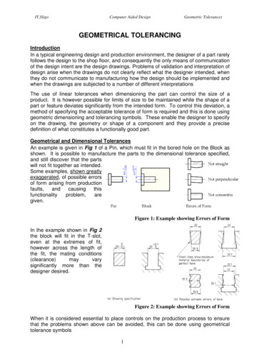
CLT:Example 1uniform population on (0,1)0.80.0 20240.00.40.60.8Weibull populationDensity4320.51.0x31.51.00.0 0.2 0.4 0.6 0.8a log normal ity0.41.2standard normal population0.00.51.01.52.02.53.03.5x48

CLT:Example 20.200.150.100.050.00Density0.250.30Central Limit Theorem at Work 20246x1 x2 x3 x49

CLT:Example 3 20240.00.20.40.6x1x2a log normal populationWeibull population0.81.000.40.02Density40.8 4Density0.60.00.2Density0.41.2uniform population on (0,1)0.0Densitystandard normal 0.0Density0.8Weibull population0.00.51.01.52.02.53.03.5x510

CLT:Example 40.00 0.15 0.30DensityCentral Limit Theorem at Work 20246x1 x2 x3 x40.0 0.2 0.4DensityCentral Limit Theorem at Work1234567x2 x3 x4 x511

CLT:Example 5uniform population on (0,1)0.80.0 20240.00.20.40.60.8x1x2a log normal populationWeibull population1.00.40.00.00.2Density0.40.8 4Density0.4Density0.20.0Density0.41.2standard normal population0510x3150.00.51.01.52.02.53.0x412

CLT:Example 60.100.050.00Density0.150.20Central Limit Theorem at Work (not so good)010203040x1 x2 x3 x413

CLT:Example 7uniform population on rd normal population 2024051015x1x2a log normal populationWeibull population200.4Density320.010Density40.85 40.00.51.0x31.50.00.51.01.52.02.53.03.5x414

CLT:Example 80.040.020.00Density0.060.08Central Limit Theorem at Work (not so good) 20 10010203040x1 x2 x3 x415

What is a Tolerance? Tolerances recognize that part dimensions are not what they should be.“should be” nominal or exact according to engineering designExact dimensions allow mass production assembly using interchangeable parts Variations around nominal are controlled by tolerances. Typical two-sided specification:[Nominal Tolerance, Nominal Tolerance] Specifications can be one-sided:[Nominal, Nominal Tolerance]or[Nominal Tolerance, Nominal ] Specifications can be asymmetric: [Nominal Tolerance1, Nominal Tolerance2]16

Simple Examples Example 1: A disk should have thickness 1/800 with .00100 tolerance, i.e.,the disk thickness should be in the range[.12500 .00100, .12500 .00100] [.12400, .12600] . Example 2: A stack of ten disks should be 1.2500 high with .0100 tolerance,i.e., the stack height should be in the range[1.2500 .0100, 1.2500 .0100] [1.2400, 1.2600] .17

Disk Stack1 8″″ 0.125 0.001″″1.25″″ 0.01″″18

Worst Case or Arithmetic Tolerancing The tolerance specification in Example 1, if adhered to,guarantees the tolerance specification in Example 2. The reasoning is based on worst case or arithmetic tolerancing The stack is highest when all disks are as thick as possible.12600 per disk stack height of 10 .12600 1.2600. The stack is lowest when all disks are as thin as possible.12400 per disk stack height of 10 .12400 1.2400. This gives the total possible stack height range as [1.2400, 1.2600] .19

disk stack/tolerance stackworst caselow stack.02''worst casehigh stack.125''1.25''20

Worst Case or Arithmetic Tolerancing in Reverse This reasoning can be reversed. If the stack height has specified end tolerance .0100,and if the disk tolerances are to be the same for all disks (exchangeable),then we should, by the worst case tolerancing reasoning, assign .0100/10 .00100tolerances to the individual disks (item tolerances). End tolerances can create very tight and unrealistic item tolerances. Costly!21

Worst Case Analysis or Goal Post Mentalitynominal tolnominal tolnominal tol-?Add some structure, aim for the middle Statistical Tolerancing22

Statistical Tolerancing Assumption Statistical tolerancing assumes that disks are chosen at random,not deliberately to make a worst possible stack, one way or the other. The disk thickness variation within tolerances is described by a distribution. The histogram, summarizing these thicknesses, is often assumed to be normal or Gaussian with center µD at the middle of the tolerance rangeand with standard deviation such that 3 standard deviations tolerance .or1σD TOLD so that [µD 3σD, µD 3σD] tolerance interval3 The normality assumption is a simplification, but is not essential.23

Normal Histogram/Distribution of Disk Thicknesses1200Histogram of 10,000 35% 0.123516 0.1240 0.12450.12500.12550.12600.1265disk thickness24

Why Does Statistical Tolerancing Work Under the normal population model we will see about 13.5 out of 10, 000disks with thickness .12600 . The chance of randomly selecting such a fat or fatter disk is .00135 13.5/10, 000 The chance of having such bad (thick) luck ten times in a row is.00135 . . . .00135 (.00135)10 2.01 10 29 (!!!) Choosing thicknesses at random from this normal population we (justifiably)hope that thick and thin will average out to some extent. Make independent variation work for you, not against you!If life gives you lemons, make lemonade! Turn a negative into a positive!25

The Insurance Principle of Averaging We look forward to the day when everyone will receivemore than the average wage.Australian Minister of Labour, 1973 The etymology of “average” derives from the Arabic: awārı̄yahmeaning shipwreck, damaged goods, and linking it to the customof averaging the losses of damaged cargo across all merchants You get the good with the bad “Havarie” in German means: shipwreck “Awerij” in Dutch/Afrikaans means: average, damage to ship or cargo26

Distribution of Stack Heights Choosing many stacksS D1 . . . D10 of ten disks eachwe get a normal population of stack heights, with mean E(S) E(D1) . . . E(D10) 10 .12500 1.2500, and standard deviationq 22σS σD1 . . . σD10 10 σD 10 .00100/3 .0010500 thus S ranges over 0000001.25 3 10 .001 /3 1.25 10 .00100 1.2500 .0031600.0031600 10 .00100 10 .00100 .010027

Normal Histogram/Distribution of Stacks2001000Density300400Histogram of 10,000 Stack Heights1.2401.2451.2501.2551.260stack height of 10 disks28

Root Sum Square (RSS) MethodFor S D1 . . . D10,σS pwith independent disk thicknesses Di,we haveqvar(D1 . . . D10) σ2D1 . . . σ2D10Interpreting TOLi TOLDi 3σDi and TOLS 3σS we haveqqTOLS 3σS 3 σ2D1 . . . σ2D10 (3σD1 )2 . . . (3σD10 )2q 22TOL1 . . . TOL10 10 TOLD µS 3σS contains 99.73% of the S values, because S N (µS , σ2S ).This is referred to as the Root Sum Square (RSS) Method of tolerance stacking.Contrast with arithmetic or worst case tolerance stackingTOL?S TOL?1 . . . TOL?10 10 TOL?D29

Some Comments on ? NotationNumerically TOLi TOL?i are the same, they are just different in what theyrepresent: statistical variation range versus worst case variation range.Again, TOLS and TOL?S represent statistical and worst case variation ranges,but they are not the same sinceqqTOL21 . . . TOL210 (TOL?1)2 . . . (TOL?10)2 TOL?1 . . . TOL?10We get only in the trivial cases whenwhenn 1andn 1orTOL1 . . . TOLn 0.30

Statistical Tolerancing Benefits stack height variation is much tighter than specified could try to relax the tolerances on the disks, relaxed tolerances lower cost of part manufacture take advantage of tighter assembly tolerances easier assembly31

RSS for General nWhen we stack n disks, replace 10 by n above: 1TOLS n TOLD or TOLD TOLSnAs opposed to the worst case tolerancing relationshipsTOL?S n TOL?Dor1?TOLD TOL?SnMore generally when the TOLDi are not all the sameTOLS qTOL21 . . . TOL2nReverse engineeringorTOLS TOLDi orTOL?S TOL?D1 . . . TOL?DnTOL?S TOL?Dinot so obvious.Reduce the largest TOLDi to get greatest impact on TOLS . TOL?D ?i32

RSS Pythagorean Shortcut. . . . . . . . . . . . .

Statistical Tolerancing Assumption Statistical tolerancing assumes that disks are chosen at random, not deliberately to make a worst possible stack, one way or the other. The disk thickness variation within tolerances is described by a distribution. The histogram, summarizing these thicknesses, is often assumed to be normal or Gaussian with center µD at the middle of the .