Transcription
Regularized M -estimators with nonconvexity:Statistical and algorithmic theory for local optimaMartin J. WainwrightDepartments of Statistics and EECSUniversity of California, BerkeleyBerkeley, CA 94720wainwrig@stat.berkeley.eduPo-Ling LohDepartment of StatisticsUniversity of California, BerkeleyBerkeley, CA 94720ploh@berkeley.eduAbstractWe establish theoretical results concerning local optima of regularized M estimators, where both loss and penalty functions are allowed to be nonconvex.Our results show that as long as the loss satisfies restricted strong convexity andthe penalty satisfies suitable regularity conditions, any local optimum of the composite objective lies within statistical precision of the true parameter vector. Ourtheory covers a broad class of nonconvex objective functions, including correctedversions of the Lasso for errors-in-variables linear models and regression in generalized linear models using nonconvex regularizers such as SCAD and MCP. Onthe optimization side, we show that a simple adaptation of composite gradient descent may be used to compute a global optimum up to the statistical precision statin log(1/ stat ) iterations, the fastest possible rate for any first-order method. Weprovide simulations to illustrate the sharpness of our theoretical predictions.1IntroductionOptimization of nonconvex functions is known to be computationally intractable in general [11, 12].Unlike convex functions, nonconvex functions may possess local optima that are not global optima,and standard iterative methods such as gradient descent and coordinate descent are only guaranteedto converge to local optima. Although statistical results regarding nonconvex M -estimation oftenonly provide guarantees about the accuracy of global optima, it is observed empirically that the localoptima obtained by various estimation algorithms seem to be well-behaved.In this paper, we study the question of whether it is possible to certify “good” behavior, in both astatistical and computational sense, for various nonconvex M -estimators. On the statistical level,we provide an abstract result, applicable to a broad class of (potentially nonconvex) M -estimators,which bounds the distance between any local optimum and the unique minimum of the populationrisk. Although local optima of nonconvex objectives may not coincide with global optima, ourtheory shows that any local optimum is essentially as good as a global optimum from a statisticalperspective. The class of M -estimators covered by our theory includes the modified Lasso as aspecial case, but our results are much stronger than those implied by previous work [6].In addition to nonconvex loss functions, our theory also applies to nonconvex regularizers, sheddingnew light on a long line of recent work involving the nonconvex SCAD and MCP regularizers [3, 2,13, 14]. Various methods have been proposed for optimizing convex loss functions with nonconvexpenalties [3, 4, 15], but these methods are only guaranteed to generate local optima of the compositeobjective, which have not been proven to be well-behaved. In contrast, our work provides a setof regularity conditions under which all local optima are guaranteed to lie within a small ball ofthe population-level minimum, ensuring that standard methods such as projected and compositegradient descent [10] are sufficient for obtaining estimators that lie within statistical error of the1
truth. In fact, we establish that under suitable conditions, a modified form of composite gradientdescent only requires log(1/ stat ) iterations to obtain a solution that is accurate up to the statisticalprecision stat .Notation. For functions f (n) and g(n), we write f (n) - g(n) to mean that f (n) cg(n) forsome universal constant c (0, ), and similarly, f (n) % g(n) when f (n) c0 g(n) for someuniversal constant c0 (0, ). We write f (n) g(n) when f (n) - g(n) and f (n) % g(n) holdsimultaneously. For a function h : Rp R, we write h to denote a gradient or subgradient, if itexists. Finally, for q, r 0, let Bq (r) denote the q -ball of radius r centered around 0.2Problem formulationIn this section, we develop some general theory for regularized M -estimators. We first establishnotation, then discuss assumptions for nonconvex regularizers and losses studied in our paper.2.1BackgroundGiven a collection of n samples Z1n {Z1 , . . . , Zn }, drawn from a marginal distribution P over aspace Z, consider a loss function Ln : Rp (Z)n R. The value Ln (β; Z1n ) serves as a measureof the “fit” between a parameter vector β Rp and the observed data. This empirical loss functionshould be viewed as a surrogate to the population risk function L : Rp R, given by L(β) : EZ Ln (β; Z1n ) .Our goal is to estimate the parameter vector β : arg minp L(β) that minimizes the populationβ Rrisk, assumed to be unique.To this end, we consider a regularized M -estimator of the formβb arg min {Ln (β; Z1n ) ρλ (β)} ,g(β) R(1)where ρλ : Rp R is a regularizer, depending on a tuning parameter λ 0, which serves toenforce a certain type of structure on the solution. In all cases, we consider regularizersthat arePpseparable across coordinates, and with a slight abuse of notation, we write ρλ (β) j 1 ρλ (βj ).Our theory allows for possible nonconvexity in both the loss function Ln and the regularizer ρλ .Due to this potential nonconvexity, our M -estimator also includes a side constraint g : Rp R ,which we require to be a convex function satisfying the lower bound g(β) kβk1 , for all β Rp .Consequently, any feasible point for the optimization problem (1) satisfies the constraint kβk1 R,and as long as the empirical loss and regularizer are continuous, the Weierstrass extreme valuetheorem guarantees that a global minimum βb exists.2.2Nonconvex regularizersWe now state and discuss conditions on the regularizer, defined in terms of ρλ : R R.Assumption 1.(i) The function ρλ satisfies ρλ (0) 0 and is symmetric around zero (i.e., ρλ (t) ρλ ( t)for all t R).(ii) On the nonnegative real line, the function ρλ is nondecreasing.(iii) For t 0, the function t 7 ρλ (t)tis nonincreasing in t.(iv) The function ρλ is differentiable for all t 6 0 and subdifferentiable at t 0, with nonzerosubgradients at t 0 bounded by λL.(v) There exists µ 0 such that ρλ,µ (t) : ρλ (t) µt2 is convex.Many regularizers that are commonly used in practice satisfy Assumption 1, including the 1 -norm,ρλ (β) kβk1 , and the following commonly used nonconvex regularizers:2
SCAD penalty: This penalty, due to Fan and Li [3], takes the form for t λ, λ t ,22ρλ (t) : (t 2aλ t λ )/(2(a 1)), for λ t aλ, (a 1)λ2 /2,for t aλ,where a 2 is a fixed parameter. Assumption 1 holds with L 1 and µ (2)1a 1 .MCP regularizer: This penalty, due to Zhang [13], takes the formZ t z 1 ρλ (t) : sign(t) λ ·dz,λb 0(3)where b 0 is a fixed parameter. Assumption 1 holds with L 1 and µ 1b .2.3Nonconvex loss functions and restricted strong convexityThroughout this paper, we require the loss function Ln to be differentiable, but we do not require itto be convex. Instead, we impose a weaker condition known as restricted strong convexity (RSC).Such conditions have been discussed in previous literature [9, 1], and involve a lower bound on theremainder in the first-order Taylor expansion of Ln . In particular, our main statistical result is basedon the following RSC condition: log p 2 k k21 , k k2 1,(4a) α1 k k2 τ1n rh Ln (β ) Ln (β ), i α2 k k2 τ2 log p k k1 , k k2 1,(4b)nwhere the αj ’s are strictly positive constants and the τj ’s are nonnegative constants.To understand this condition, note that if Ln were actually strongly convex, then both these RSCinequalities would hold with α1 α2 0 and τ1 τ2 0. However, in the high-dimensionalsetting (p n), the empirical loss Ln can never be strongly convex, but the RSC condition maystill hold with strictly positive (αj , τj ). On the other hand, if Ln is convex (but not strongly convex),the left-hand expressionq in inequality (4) is alwaysq nonnegative, so inequalities (4a) and (4b) holdk k1α1 nα2n1trivially for k k andk k2τ1 log pk k2τ2log p , respectively. Hence, the RSC inequalitiesnoqn1only enforce a type of strong convexity condition over a cone set of the form k k ck k2log p .3Statistical guarantees and consequencesWe now turn to our main statistical guarantees and some consequences for various statistical models.Our theory applies to any vector βe Rp that satisfies the first-order necessary conditions to be alocal minimum of the program (1):e ρλ (β),e β βie 0,h Ln (β)for all feasible β Rp .(5)When βe lies in the interior of the constraint set, condition (5) is the usual zero-subgradient condition.3.1Main statistical resultsOur main theorem is deterministic in nature, and specifies conditions on the regularizer, loss function, and parameters, which guarantee that any local optimum βe lies close to the target vectorβ arg minp L(β). Corresponding probabilistic results will be derived in subsequent sections. Forβ Rproofs and more detailed discussion of the results contained in this paper, see the technical report [7].Theorem 1. Suppose the regularizer ρλ satisfies Assumption 1, Ln satisfies the RSC conditions (4)with α1 µ, and β is feasible for the objective. Consider any choice of λ such that()r2α2log p · max k Ln (β )k , α2 λ ,(6)Ln6RL3
22216R max(τ1 ,τ2 )log p. Then any vector βe satisfying the first-order necessary conand suppose n α22ditions (5) satisfies the error bounds 7λL k56λLk ekβ β k2 ,andkβe β k1 ,(7)4(α1 µ)4(α1 µ)where k kβ k0 .From the bound (7), note that the squared 2 -error grows proportionally with k, the number of non2zeros in the targetq parameter, and with λ . As will be clarified in the following sections, choosing λproportional tolog pnand R proportional to1λwill satisfy the requirements of Theorem 1 w.h.p. formany statistical models, in which case we have a squared 2 -error that scales ask log pn ,as expected.Remark 1. It is worthwhile to discuss the quantity α1 µ appearing in the denominator of thebound in Theorem 1. Recall that α1 measures the level of curvature of the loss function Ln , while µmeasures the level of nonconvexity of the penalty ρλ . Intuitively, the two quantities should play opposing roles in our result: Larger values of µ correspond to more severe nonconvexity of the penalty,resulting in worse behavior of the overall objective (1), whereas larger values of α1 correspond tomore (restricted) curvature of the loss, leading to better behavior.We now develop corollaries for various nonconvex loss functions and regularizers of interest.3.2Corrected linear regressionWe begin by considering the case of high-dimensional linear regression with systematically corrupted observations. Recall that in the framework of ordinary linear regression, we have the modelyi hβ , xi i i , {z }Ppj 1for i 1, . . . , n,(8)βj xijwhere β Rp is the unknown parameter vector and {(xi , yi )}ni 1 are observations. Following Lohand Wainwright [6], assume we instead observe pairs {(zi , yi )}ni 1 , where the zi ’s are systematicallycorrupted versions of the corresponding xi ’s. Some examples include the following:(a) Additive noise: Observe zi xi wi , where wi xi , E[wi ] 0, and cov[wi ] Σw .(b) Missing data: For ϑ [0, 1), observe zi Rp such that for each component j, we independently observe zij xij with probability 1 ϑ, and zij with probability ϑ.We use the population and empirical loss functionsL(β) 1 Tβ Σx β β T Σx β,2andLn (β) 1 Tbβ Γβ γbT β,2(9)b γwhere (Γ,b) are estimators for (Σx , Σx β ) depending on {(zi , yi )}ni 1 . Then β arg minβ L(β).From the formulation (1), the corrected linear regression estimator is given by 1 Tbβb arg minβ Γβ γbT β ρλ (β) .(10)g(β) R 2We now state a corollary in the case of additive noise (model (a)), where we takeTb Z Z Σw ,Γnandγb ZT y.n(11)b in equation (11) is always negative-definite, so the empirical loss functionWhen p n, the matrix Γb are applicable to missing data (modelLn previously defined (9) is nonconvex. Other choices of Γ(b)), and also lead to nonconvex programs [6].4
Corollary 1. Suppose we have i.i.d. observations {(zi , yi )}ni 1 from a corrupted linear model withsub-Gaussian additive noise. Suppose (λ, R) are chosen such that β is feasible andrlog pc0c λ .nRThen given a sample size n C max{R2 , k} log p, any local optimum βe of the nonconvex program (10) satisfies the estimation error bounds c00 λkc0 λ k e,andkβe β k1 ,kβ β k2 λmin (Σx ) 2µλmin (Σx ) 2µwith probability at least 1 c1 exp( c2 log p), where kβ k0 k.q Remark 2. When ρλ (β) λkβk1 and g(β) kβk1 , taking λ logn p and R b0 k for someconstant b0 kβ k2 yields the required scaling n % k log p. Hence, the bounds in Corollary 1agree with bounds in Theorem 1 of Loh and Wainwright [6]. Note, however, that the latter resultsare stated only for a global minimum βb of the program (10), whereas Corollary 1 is a much strongere Theorem 2 of our earlier paper [6] provides an indirectresult holding for any local minimum β.route for establishing similar bounds on kβe β k1 and kβe β k2 , since the projected gradientdescent algorithm may become stuck in local minima. In contrast, our argument here does not relyon an algorithmic proof and applies to a more general class of (possibly nonconvex) penalties.Corollary 1 also has important consequences in the case where pairs {(xi , yi )}ni 1 from the linearmodel (8) are observed without corruption and ρλ is nonconvex. Then the empirical loss Ln isequivalent to the least-squares loss, modulo a constant factor. Much existing work [3, 14] onlyestablishes statistical consistency of global minima and then provides specialized algorithms forobtaining specific local optima that are provably close to global optima. In contrast, our resultsdemonstrate that any optimization algorithm converging to a local optimum suffices.3.3Generalized linear modelsMoving beyond linear regression, we now consider the case where observations are drawn from ageneralized linear model (GLM). Recall that a GLM is characterized by the conditional distribution yi hβ, xi i ψ(xTi β)P(yi xi , β, σ) exp,c(σ)where σ 0 is a scale parameter and ψ is the cumulant function. By standard properties of exponential families [8, 5], we haveψ 0 (xTi β) E[yi xi , β, σ].In our analysis, we assume there exists αu 0 such that ψ 00 (t) αu for all t R. This boundedness assumption holds in various settings, including linear regression, logistic regression, andmultinomial regression. The bound is required to establish both statistical consistency results in thepresent section and fast global convergence guarantees for our optimization algorithms in Section 4.We will assume that β is sparse and optimize the penalized maximum likelihood program)( nX 1TTψ(xi β) yi xi β ρλ (β) .βb arg minn i 1g(β) R(12)We then have the following corollary:Corollary 2. Suppose we have i.i.d. observations {(xi , yi )}ni 1 from a GLM, where the xi ’s aresub-Gaussian. Suppose (λ, R) are chosen such that β is feasible andrc0log pc λ .nR2eGiven a sample size n CR log p, any local optimum β of the nonconvex program (12) satisfies c0 λ kc00 λk ekβ β k2 ,andkβe β k1 ,λmin (Σx ) 2µλmin (Σx ) 2µwith probability at least 1 c1 exp( c2 log p), where kβ k0 k.5
4Optimization algorithmWe now describe how a version of composite gradient descent may be applied to efficiently optimizethe nonconvex program (1). We focus on a version of the optimization problem with the side functiono1ngλ,µ (β) : (13)ρλ (β) µkβk22 ,λwhich is convex by Assumption 1. We may then write the program (1) asno βb arg minLn (β) µkβk22 λgλ,µ (β) .(14)gλ,µ (β) R {z}L̄nThe objective function then decomposes nicely into a sum of a differentiable but nonconvex functionand a possibly nonsmooth but convex penalty. Applied to the representation (14), the compositegradient descent procedure of Nesterov [10] produces a sequence of iterates {β t } t 0 via the updates() 2t Lλ(β)1nβ βt gλ,µ (β) ,β t 1 arg min(15)2ηηgλ,µ (β) R2where1ηis the stepsize. Define the Taylor error around β2 in the direction β1 β2 byT (β1 , β2 ) : Ln (β1 ) Ln (β2 ) h Ln (β2 ), β1 β2 i.(16)For all vectors β2 B2 (3) B1 (R), we require the following form of restricted strong convexity: log p 2 kβ1 β2 k21 , kβ1 β2 k2 3,(17a) α1 kβ1 β2 k2 τ1nrT (β1 , β2 ) α2 kβ1 β2 k2 τ2 log p kβ1 β2 k1 , kβ1 β2 k2 3.(17b)nThe conditions (17) are similar but not identical to the earlier RSC conditions (4). The maindifference is that we now require the Taylor difference to be bounded below uniformly overβ2 B2 (3) B1 (R), as opposed to for a fixed β2 β . We also assume an upper bound:log pT (β1 , β2 ) α3 kβ1 β2 k22 τ3kβ1 β2 k21 ,for all β1 , β2 Rp ,(18)na condition referred to as restricted smoothness in past work [1]. Throughout this section, we assume αi µ for all i, where µ is the coefficient ensuring the convexity of the function gλ,µ fromequation (13). Furthermore, we define α min{α1 , α2 } and τ max{τ1 , τ2 , τ3 }.The following theorem applies to any population loss function L for which the population minimizerβ is k-sparse and kβ k2 1, and under the scaling n Ck log p, for a constant C depending onthe αi ’s and τi ’s. We show that the composite gradient updates (15) exhibit a type of globallygeometric convergence in terms of the quantityα µ4η128τ k logn p.1 ϕ(n, p, k)α µUnder the stated scaling on the sample size, we are guaranteed that κ (0, 1). Let 0 bβ) 2 log φ(β ) φ(δ2log 2λRL T (δ) : 1 log log,log(1/κ)log(1/κ)δ2where φ(β) : Ln (β) ρλ (β), and define stat : kβb β k2 .κ : 1 ϕ(n, p, k),where ϕ(n, p, k) : (19)(20)Theorem 2. Suppose Ln satisfies the RSC/RSM conditions (17) and (18), and suppose ρλ satisfiesAssumption 1. Suppose βb is any global minimum of the program (14), with()rrlog p4log p R c,andλ · max k Ln (β )k , τ.nLnc 2statThen for any stepsize η 2 · max{α3 µ, µ} and tolerance δ 2 1 κ, we have 42δk log p 2b 2 kβ t βkδ2 128τ stat , t T (δ).2α µτn6(21)
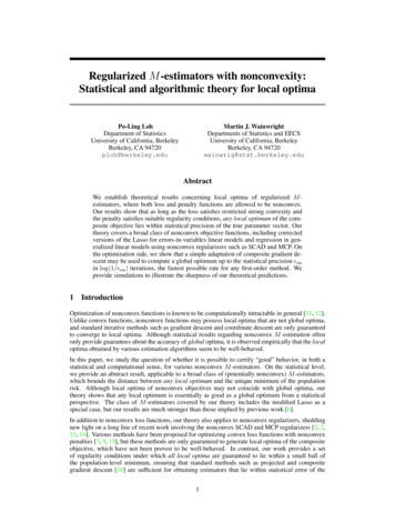
Remark 3. Note that for the optimal choice of tolerance parameter δ stat , the bound in inequalc 2statity (21) takes the form α µ, meaning successive iterates are guaranteed to converge to a regionb Combining Theorems 1 and 2, we havewithin statistical accuracy of the true global optimum β.!rnok log ptt b, t T (c0 stat ).max kβ βk2 , kβ β k2 On5SimulationsIn this section, we report the results of simulations for two versions of the loss function Ln , corresponding to linear and logistic regression, and three penalty functions: Lasso,q SCAD, and MCP. Inall cases, we chose regularization parameters R 1.1λ· ρλ (β ) and λ log pn .Linear regression: In the case of linear regression, we simulated covariates corrupted by additivenoise according to the mechanism described in Section 3.2, giving the estimator 1 T XT XyT Zβb arg minβ Σw β β ρλ (β) .(22)nngλ,µ (β) R 2We generated i.i.d. samples xi N (0, I) and i N (0, (0.1)2 ), and set Σw (0.2)2 I.Logistic regression: In the case of logistic regression, we generated i.i.d. samples xi N (0, I).Since ψ(t) log(1 exp(t)), the program (12) becomes)( nX1{log(1 exp(hβ, xi i) yi hβ, xi i} ρλ (β) .(23)βb arg minn i 1gλ,µ (β) RWe optimized the programs (22) and (23) using the composite gradient updates (15). Figure 1shows the results of corrected linear regression with Lasso, SCAD, and MCP regularizers for threedifferent problem sizes p. In each case, β is a k-sparse vector with k b pc, where the nonzeroentries were generated from a normal distribution and the vector was then rescaled so kβ k2 1.As predicted by Theorem 1, the curves corresponding to the same penalty function stack up nicelynwhen the estimation error kβb β k2 is plotted against the rescaled sample size k logp , and the 2 error decreases to zero as the number of samples increases, showing that the estimators (22) and (23)are statistically consistent. We chose the parameter a 3.7 for SCAD and b 3.5 for MCP.comparing penalties for corrected linear regression0.50.30.20.100p 128p 256p 5120.9l2 norm error0.4l2 norm errorcomparing penalties for logistic regression1p 128p 256p 5120.80.70.60.5102030n/(k log p)400.4050(a)204060n/(k log p)80100(b)Figure 1. Plots showing statistical consistency of (a) linear and (b) logistic regression with Lasso,SCAD, and MCP. Each point represents an average over 20 trials. The estimation error kβb β k2nis plotted against the rescaled sample size k log. Lasso, SCAD, and MCP results are represented bypsolid, dotted, and dashed lines, respectively.The simulations in Figure 2 depict the optimization-theoretic conclusions of Theorem 2. Each panelshows two different families of curves, corresponding to statistical error (red) and optimization error7
(blue). The vertical axis measures the 2 -error on a log scale, while the horizontal axis tracks theiteration number. The curves were obtained by running composite gradient descent from 10 randomstarting points. We used p 128, k b pc, and n b20k log pc. As predicted by our theory,the optimization error decreases at a linear rate until it falls to the level of statistical error. Panels(b) and (c) provide simulations for two values of the SCAD parameter a; the larger choice a 3.7corresponds to a higher level of curvature and produces a tighter cluster of local optima.log error plot for corrected linear regression with MCP, b 1.52opt errstat err0log error plot for corrected linear regression with SCAD, a 3.72opt errstat err0log error plot for corrected linear regression with SCAD, a 2.51opt errstat err0 2 2 1 8 2) 3t 4log( 6log( log( tt * 4* 2)* 2) 2 6 4 5 6 8 10 120200400600iteration count800 1001000 7200400(a)600800iteration count1000 801200200400(b)600800iteration count10001200(c)Figure 2. Plots illustrating linear rates of convergence for corrected linear regression with MCP and SCAD. Red lines depict statistical error log kβb β k2 and blue lines depict optimization error b 2 . As predicted by Theorem 2, the optimization error decreases linearly up to statisticallog kβ t βkaccuracy. Each plot shows the solution trajectory for 10 initializations of composite gradient descent.Panel (a) shows results for MCP; panels (b) and (c) show results for SCAD with different values of a. Figure 3 provides analogous results to Figure 2 for logistic regression, using p 64, k b pc, andn b20k log pc. The plot shows solution trajectories for 20 different initializations of compositegradient descent. Again, the log optimization error decreases at a linear rate up to the level ofstatistical error, as predicted by Theorem 2. Whereas the convex Lasso penalty yields a uniqueb SCAD and MCP produce multiple local optima.local/global optimum β,log error plot for logistic regression with Lasso1log error plot for logistic regression with SCAD, a 3.70.5opt errstat err0 2) 1 65001000iteration count(a)15002000 1.5t 5 70 1.5t 2log( log( tlog( 4 1* 2) 0.5**2 ) 3opt errstat err0 0.5 1 2log error plot for logistic regression with MCP, b 30.5opt errstat err0 2.5 2 2.5 3 3 3.5 3.5 405001000iteration count(b)15002000 405001000iteration count15002000(c)Figure 3. Plots showing linear rates of convergence on a log scale for logistic regression. Red linesdepict statistical error and blue lines depict optimization error. (a) Lasso penalty. (b) SCAD penalty.(c) MCP. Each plot shows the solution trajectory for 20 initializations of composite gradient descent.6DiscussionWe have analyzed theoretical properties of local optima of regularized M -estimators, where boththe loss and penalty function are allowed to be nonconvex. Our results are the first to establish thatall local optima of such nonconvex problems are close to the truth, implying that any optimizationmethod guaranteed to converge to a local optimum will provide statistically consistent solutions. Weshow that a variant of composite gradient descent may be used to obtain near-global optima in lineartime, and verify our theoretical results with simulations.AcknowledgmentsPL acknowledges support from a Hertz Foundation Fellowship and an NSF Graduate Research Fellowship. MJW and PL were also partially supported by grants NSF-DMS-0907632 and AFOSR09NL184. The authors thank the anonymous reviewers for helpful feedback.8
References[1] A. Agarwal, S. Negahban, and M. J. Wainwright. Fast global convergence of gradient methodsfor high-dimensional statistical recovery. Annals of Statistics, 40(5):2452–2482, 2012.[2] P. Breheny and J. Huang. Coordinate descent algorithms for nonconvex penalized regression,with applications to biological feature selection. Annals of Applied Statistics, 5(1):232–253,2011.[3] J. Fan and R. Li. Variable selection via nonconcave penalized likelihood and its oracle properties. Journal of the American Statistical Association, 96:1348–1360, 2001.[4] D. R. Hunter and R. Li. Variable selection using MM algorithms. Annals of Statistics,33(4):1617–1642, 2005.[5] E.L. Lehmann and G. Casella. Theory of Point Estimation. Springer Verlag, 1998.[6] P. Loh and M.J. Wainwright. High-dimensional regression with noisy and missing data: Provable guarantees with non-convexity. Annals of Statistics, 40(3):1637–1664, 2012.[7] P. Loh and M.J. Wainwright. Regularized M -estimators with nonconvexity: Statistical andalgorithmic theory for local optima. arXiv e-prints, May 2013. Available at http://arxiv.org/abs/1305.2436.[8] P. McCullagh and J. A. Nelder. Generalized Linear Models (Second Edition). London: Chapman & Hall, 1989.[9] S. Negahban, P. Ravikumar, M. J. Wainwright, and B. Yu. A unified framework for highdimensional analysis of M -estimators with decomposable regularizers. Statistical Science,27(4):538–557, December 2012. See arXiv version for lemma/propositions cited here.[10] Y. Nesterov. Gradient methods for minimizing composite objective function. CORE Discussion Papers 2007076, Universit Catholique de Louvain, Center for Operations Research andEconometrics (CORE), 2007.[11] Y. Nesterov and A. Nemirovskii. Interior Point Polynomial Algorithms in Convex Programming. SIAM studies in applied and numerical mathematics. Society for Industrial and AppliedMathematics, 1987.[12] S. A. Vavasis. Complexity issues in global optimization: A survey. In Handbook of GlobalOptimization, pages 27–41. Kluwer, 1995.[13] C.-H. Zhang. Nearly unbiased variable selection under minimax concave penalty. Annals ofStatistics, 38(2):894–942, 2010.[14] C.-H. Zhang and T. Zhang. A general theory of concave regularization for high-dimensionalsparse estimation problems. Statistical Science, 27(4):576–593, 2012.[15] H. Zou and R. Li. One-step sparse estimates in nonconcave penalized likelihood models.Annals of Statistics, 36(4):1509–1533, 2008.9
3 Statistical guarantees and consequences We now turn to our main statistical guarantees and some consequences for various statistical models. Our theory applies to any vector pe2R that satisfies the first-order necessary conditions to be a local minimum of the program (1