Transcription
A Survey of High-Frequency TradingStrategiesBrandon Beckhardt1 , David Frankl2 , Charles Lu3 , and du3charleslu@stanford.edu4mkwang@stanford.edu2June 6, 2016AbstractWe survey and implement a number of known high frequency trading strategies. These strategies take advantages of Thesys high frequency data and attempt to trade intraday from frequencies rangingfrom milliseconds to minutes, some utilizing machine learning techniques. While discussing and implementing these strategies was insightful, we fail to make significant profit after accounting for transaction costs. That is not to say these strategies do not work in general.We also hope to elucidate where our strategies fall short and where toimprove them.0BB contributed the correlation model strategy. DF contributed the ETF statisticalarbitrage strategy. CL contributed the order book pressure strategy. MW contributedthe automated technical strategy search and intelligent market making algorithm. Wethank Lisa Borland and Enzo Busseti for all the insightful discussions and trading ideas.We would also like to thank Artem Vasilyev for contributing his deep insight on ”recurrent neural networks” and ”locality sensitive hashing” for instantaneous exchange latencyarbitrage. Finally, Thesys provided the equity data.1
1IntroductionIn this paper, we will present five different high frequency trading strategiesthat we researched and implemented using Thesys data and platform. Thestrategies are diverse in nature and attempt to capitalize on independentsources of alpha. So, our original intent was to combine such independentpredictors into one ensemble trading strategy. However, in our case, a fullensemble proves to be needlessly complex. Alternatively, we can propose tocombine our strategies (once they are tuned and profitable) with Markowitzportfolio optimization.As a result, we decided to individual research and implement five strategies. The first is a method to search for and identify profitable technicalanalysis strategies that do not overfit. Next, we attempt to statistically arbitrage highly correlated index tracking ETFs. In a similar vein, anotherstrategy models correlation between assets and attempts to profit off assetdivergence. Fourth, a strategy to predict price movements from order bookpressure dynamics tuned with machine learning techniques manages to turna profit. Finally, we have an intelligent market making strategy that placesits quotes based on a machine learning algorithm trained on order book dynamics.2Data and MethodsSince Thesys only provides equity data, our universe of assets are limited tostocks. We choose equities listed on SP500, NASDAQ, and NYSE becausethey are liquid to facilitate high frequency trading. Code and simulations arerun within Thesys’s platform, which is hosted on a Jupyter notebook. Weutilized Python packages such as Pandas, NumPy, and scikit-learn for ourquantitative analysis.33.1Strategy 1: Automated Technical StrategySearchBackgroundThis ”strategy” is less of an algorithmic per se but rather a technique forfinding profitable technical analysis strategies, which can then be turnedinto algorithms. The goal is to define a strategy space - a set of a certain2
enumerable strategy type - and search over that space, selecting only themost profitable for trading.With a naive approach, the primary issue is overfitting. Since we onlyhave historical data with which to search (and select our strategies from),it is possible and indeed highly probable that we select spurious technicalanalysis signals that look like they have predictive power but perform quitepoorly out of sample. In real world trading, this issue becomes a strongconcern for technical traders, who psychologically believe they identify profitable patterns on historical data, but rack up huge losses when using thesame patterns on forward trading. To mitigate this concern, we seek to finda way to systematically address the issue of overfitting.This technique was inspired by that of a hedge fund manager JaffrayWoodriff of Quantitative Investment Management.[7] While not much is extensively known about his specific technique, it is know that Woodriff employs random time series in searching for technical analysis strategies andthat he combines his technical predictors into an ensemble.[6] Additionalhelp was obtained through a blog post attempting to replicate Woodriff’smethods. We extend their work on lower frequency daily data to high frequency tick and order book data.3.2Benchmarking on Random DataTo this end, we come up with the approach to benchmark the strategies in ourstrategies against their performance on random time series data. The goalwe have in mind is to select the highest returning strategies in our strategyspace that aren’t overfit or due to random noise. On random data, we trythe strategies on our strategy space and achieve some baseline returns. Sincethe underlying time series are random, we know even the best performing ofthese strategies have zero alpha.So when we run the same strategies on real time series data, the oneshere that outperform those on random data will have positive alpha. Fromthis, we conclude that these top performers on real data that beat those onfake data turn significant profit as to be not overfit or due to random noise.3.3Generating Realistic Random Time SeriesThe insight here was to employ the bootstrap, a statistical technique forsampling with replacement.First, we obtain a day’s worth of tick data (bid and ask quotes) for asingle stock of interest in our universe. This leads to around one milliondifferent tick events which include all changes at the inside order book. For3
computation simplicity, we then compute each tick’s price change as an absolute difference (assumed due to the fine granularity of the returns) in midmarket price.Next, we use the full day’s mid market price changes and the time betweeneach tick to produce two empirical probability distribution functions (PDFs).So, we come up with an algorithm to generate and simulated random walk.First, initialize t 0 and first price p0 randomly within some boundsand have a list of trade times as vector T . Furthermore have a list of pricesP . While t end of day, draw a time change tδ from the PDF and a pricechange pδ . Store these into the vectors: T tprev tδ , and P pprev pδ .Here denotes the append to vector operation.When this finishes, we will have a random walk for a day’s worth of ticksand corresponding prices modeling on the empirically observed price changesand trade times during the day. In essence, we have shaken up the originalday’s events on two axes: the price and time. This procedure allows us torapidly generate realistic looking random price time series.In apply this procedure, there’s the tacit assumption that ticks are IID,which may not be a perfect assumption. One can imagine that the information gleamed from one tick and order would affect subsequent tradesalso, thereby violating our assumption. More concretely, this assumptionmakes the produced random time series (which still realistic looking) haveless volatility clustering as expected. However, we believe this to not affectthe procedure as a whole. Because we are not doing any learning or fittingon the random data itself, we believe this assumption to be a minor flaw.This real series of real AAPL on 2015-01-21 becomes transformed into4
3.4Results on Strategy Space of 4 Tick Price ActionWe will now demonstrate the technique on a sample strategy space of all priceaction strategies of 4 ticks, looking at the sign of the price change within 4events. We arbitrary impose a holding time of 200ms (but this could be aparameter to tune). The strategy looks likeWe simply brute force over all possible strategies. There are 2 34 ofthese, since there are three outcomes at each tick 1, 0, 1 (down, neutral,and up) and two resulting actions: buy and short.The most profitable strategy on fake data performed at a profit of 2083microdollars per trade whereas the most profitable strategy (a downwardmomentum strategy!) profited 3461 microdollars per trade. So, our techniqueposits that this downward momentum technical analysis strategy is predictiveout of sample.If all the strategy are plotted on their profitability as so:we see the green line (strategies on real data) outperform those on fake5
data (blue line) so the difference is presumed alpha.3.5DiscussionThis technique looks promising though not necessarily on high frequencydata. First, technical analysis has an ambiguous underlying mechanism inthe high frequency space; it is premised on behavior inefficiencies leading toprice patterns, but when trades are dictated by algorithms and computers,do those same patterns have meaning? Additionally, trading on high frequency data requires aggressive trading, often crossing the spread to inputmarket orders, wiping out the 3046 microdollar/trade profit we attained inthe sample strategy.There are also problems with computation intractability associated withare search strategy. Right now, we are simply brute forcing and trying every possible permutation. Obviously, this will require exponentially morecomputing power as we increase the complexity of our strategy space. Onepossible iteration include a more intelligent search mechanism such as geneticalgorithms.44.1Strategy 2: Exploiting CorrelationBackgroundFinding assets that are correlated in some way, building a mathematicalmodel for this correlation, then trading based off of that correlation is common practice in many different trading strategies. We implemented a tradingstrategy that finds the correlation between two (or more) assets and trades ifthere is a strong deviation from this correlation, in a high frequency setting.The inspiration for this strategy came from the article Online Algorithms inHigh-frequency Trading The challenges faced by competing HFT algorithms,written by Jacob Loveless, Sasha Stoikov, and Rolf Waeber.4.2AlgorithmTo create a model representing the correlation between assets, we implemented an exponentially weighted linear regression. This linear regression ismeant to model the linear relationship between the asset we are looking totrade Y and the component assets X we are using to find this relationship.The resulting linear combination will be of the form:Y βX 6(1)
Y is a vector of points representing the assets price, X is a m n 1 matrixwhere m is the number of price points we are evaluating and n is the numberof assets we’re using to estimate Y . The first column of X is the interceptterm. is a vector representing the difference in prices needed to exactlymodel Y . Since our assumptions for trading are based on the differencebetween our estimate and the actual asset price, we are acutally not using ,so our resulting algorithm isEstimated Y βX(2)(X T W X) 1 (X T W Y )(3)β is calculated usingwhere Y represents the actual price points of the asset we are looking totrade. W is a diagonal matrix that is responsible for exponentially weightingour linear regression. In order to create our weighting scheme, we chose analpha between 0 and 1 and populate the diagonal matrix usingW [time step][time step] αtotal time steps time step 1 . Note that there are fasterways to compute an exponentially weighted linear regression, as noted in theACM article mentioned in the background section above, however for thisproject we choose to calculate the regression this way due to its simple implementation.4.3The ExploitOnce you can model the correlation between asset prices and find the ”lineof best fit” between the two, many options become available based on theassumptions that are made. The main assumption we based our algorithmfrom is that the asset we are trading, Y, will closely follow our regression,Estimated Y, if Y is highly correlated with the assets that are used to createthe regression. Under this assumption, if we see the price of Y deviatingfrom the price of Estimated Y, we assume that there will be a convergencein the near future. An example of this expected convergence can be foundin the figure below:7
This chart represents Exxon Mobile (XOM) vs a regression between ExxonMobile and Chevron Corporation (CVX). Unfortunately, most assets (including these two) generally don’t follow such a mean-reverting correlation,however this example taken from March 25th, 2015 highlights a trend wehoped to exploit.Our general approach for trading can be found below:This approach buys when it sees a far divergence of the asset price downward relative to the regression price, and sells when there is a high divergenceupward. The algorithm sells all assets that were most recently bought whenthe asset has almost reverted to the regression price (while moving upwards),and covers the sold assets when reverting downwards toward the regressionprice. It is important to note that we only ”Sell Bought Assets” when we are8
reverting to the regression from below the regression (in other words movingup in price), and only ”Cover Sold Assets” when reverting to the regressionfrom above the regression (in other words moving down in price). Coveringsold assets consists of buying back the assets we just sold, which simulatescovering a short. We added a ”Do Nothing” threshold because we foundthere was a lot of trades being executed with resulting profits that were toosmall to cover the bid-ask spread. The thresholds for determining when totrade will be discussed in the ”Parameter Tuning” section.This exploit can be used with many different approaches. Some of theapproaches we looked at were: Pairs Trading - this consists of trading between based on divergence andconvergence of two highly correlated assets. Many times, algorithmswill trade both assets in opposite fashions (sell one, buy the other andvice versa) however during the 10 weeks we were only able to focus onselling just one of the asse
That is not to say these strategies do not work in general. We also hope to elucidate where our strategies fall short and where to improve them. 0BB contributed the correlation model strategy. DF contributed the ETF statistical arbitrage strategy. CL contributed the order book pressure strategy. MW contributed the automated technical strategy search and intelligent market making algorithm. We .