Transcription
Introduction ayes’ RuleBayesianstatisticalinferenceBayesian inferencefor the BinomialdistributionIntroduction to Bayesian(geo)-statistical modellingProbabilitydistribution forthe eregressionSpatialBayesiananalysisReferencesD G RossiterCornell University, Soil & Crop Sciences SectionMarch 17, 2020
Introduction toBayesian(geo)-statisticalmodelling1 BackgroundDGRBackground2 Bayes’ RuleBayes’ RuleBayesianstatisticalinferenceBayesian inferencefor the BinomialdistributionProbabilitydistribution forthe eregressionSpatialBayesiananalysisReferences3 Bayesian statistical inferenceBayesian inference for the Binomial distributionProbability distribution for the binomial parameterPosterior inference4 Hierarchical models5 Multi-parameter models6 Numerical methods7 Multivariate regression8 Spatial Bayesian analysis
Introduction toBayesian(geo)-statisticalmodelling1 BackgroundDGRBackground2 Bayes’ RuleBayes’ RuleBayesianstatisticalinferenceBayesian inferencefor the BinomialdistributionProbabilitydistribution forthe eregressionSpatialBayesiananalysisReferences3 Bayesian statistical inferenceBayesian inference for the Binomial distributionProbability distribution for the binomial parameterPosterior inference4 Hierarchical models5 Multi-parameter models6 Numerical methods7 Multivariate regression8 Spatial Bayesian analysis
Introduction ackgroundBayes’ RuleBayesianstatisticalinferenceBayesian inferencefor the BinomialdistributionProbabilitydistribution forthe eregressionSpatialBayesiananalysisReferences Bayes’ 1763 paper [2]: theory of inverse probability inorder to make probabilistic statements about the future A simple use of conditional probability: “Bayes’ Rule” Later extended to statistical distributions: “Bayesian” “Bayes-like” Focus is on decision-making under uncertainty A useful way of thinking about probability. An increasingly common way of making inferences,because of its flexibility Can handle arbitrarily complex models, e.g., hierarchical Modern computing methods make this accessible
Introduction groundBayes’ RuleBayesianstatisticalinferenceBayesian inferencefor the Binomialdistribution Frequentist R A Fisher at Rothamstead Experimental Station (England),1920’s and 1930’sProbabilitydistribution forthe binomialparameter developed by well-known workers (Yates, Snedecor,Posteriorinference Common statistical computing packages follow sisReferencesCochran . . . ) Bayesian named for Thomas Bayes (1701–1761) developed since the 1960’s (Jeffreys, de Finetti, Wald,Savage, Lindley . . . ) requires sophisticated computing and complexmathematics
Introduction toBayesian(geo)-statisticalmodellingPrincipal differencesDGRBackgroundBayes’ RuleBayesianstatisticalinferenceBayesian inferencefor the BinomialdistributionProbabilitydistribution forthe eregressionSpatialBayesiananalysisReferences Interpretation of the meaning of probability Hypothesis testing Prediction Presentation of probabilistic results e.g. confidence intervals vs. credible intervals Computational methods
Introduction toBayesian(geo)-statisticalmodellingWhat is probability?DGRBackgroundBayes’ RuleBayesianstatisticalinferenceBayesian inferencefor the BinomialdistributionProbabilitydistribution forthe ntist the probability of an outcome is the proportionof experiments in which the outcome occurs, insome hypothetical repetitions of the experimentunder the same conditions and with the samepopulationBayesian subjective belief in the probability of an outcome,consistent with some axiomsIn both cases, experiments/observations of a sample are usedfor inference.
Introduction toBayesian(geo)-statisticalmodellingBayesian concept of probabilityDGRBackgroundBayes’ RuleBayesianstatisticalinferenceBayesian inferencefor the BinomialdistributionProbabilitydistribution forthe eregressionSpatialBayesiananalysisReferences the degree of rational belief that something is true; so certain rules of consistency must be followed All probability is conditional on evidence; Any statement has a probability distribution; any value of a parameter has a defined probability; Probability is continuously updated in view of newevidence. So, there is a degree of subjectivity; but this is reduced asmore evidence is accumulated.
Introduction toBayesian(geo)-statisticalmodellingTypes of probabilityDGRBackgroundBayes’ RuleBayesianstatisticalinferenceBayesian inferencefor the BinomialdistributionProbabilitydistribution forthe eregressionSpatialBayesiananalysisReferences Prior probability: before observations are made, withprevious knowledge; Posterior probability: after observations are made, usingthis new information; Unconditional probability: not taking into account otherevents, other than general knowledge and agreed-on facts; Joint probability: of two or more event(s); Conditional probability: in light of other information, i.e.,some other event(s) that may affect it.
Introduction toBayesian(geo)-statisticalmodellingDGRBayesian thinking about statisticaldistributionsBackgroundBayes’ RuleBayesianstatisticalinferenceBayesian inferencefor the BinomialdistributionProbabilitydistribution forthe eregressionSpatialBayesiananalysisReferences Parameters of statistical distributions are randomvariables, i.e., they also have their own statisticaldistributions, which in turn have parameters, often calledhyperparameters Statistical inferences are based on a posterior (“after thefact”) distribution of parameters of statistical distributions These are updated versions of prior (“before the fact”)beliefs based on data from experiments or observations. The updating depends on the likelihood of each possiblevalue of the parameters, given the data actually observed.
Introduction toBayesian(geo)-statisticalmodellingSubjectivity in Bayesian thinkingDGRBackgroundBayes’ RuleBayesianstatisticalinferenceBayesian inferencefor the BinomialdistributionProbabilitydistribution forthe eregressionSpatialBayesiananalysisReferences It is required to have prior probability distributions, set bythe analyst “Solution”: non-informative (actually, “minimum priorinformation”) priors But do we want these? In most situations we have priorevidence to incorporate in the decision-making. The selection of model form in both Bayesian andclassical approaches is subjective although the fit of the model form to the data can becompared (internal evaluation).
Introduction toBayesian(geo)-statisticalmodelling1 BackgroundDGRBackground2 Bayes’ RuleBayes’ RuleBayesianstatisticalinferenceBayesian inferencefor the BinomialdistributionProbabilitydistribution forthe eregressionSpatialBayesiananalysisReferences3 Bayesian statistical inferenceBayesian inference for the Binomial distributionProbability distribution for the binomial parameterPosterior inference4 Hierarchical models5 Multi-parameter models6 Numerical methods7 Multivariate regression8 Spatial Bayesian analysis
Introduction toBayesian(geo)-statisticalmodellingBayes’ Rule (1)DGRBackgroundBayes’ RuleBayesianstatisticalinferenceBayesian inferencefor the BinomialdistributionProbabilitydistribution forthe eregressionSpatialBayesiananalysisReferences One aspect of Bayesian computation is not controversial:Bayes’ Rule derived from the definition of conditionalprobability. P(A), P(B) unconditional probability of two events Joint probability P(A B) of two events A and B, i.e., thatboth occur. Reformulated in terms of conditional probability, i.e., thatone event occurs conditional on the other having occurred:P(A B) P(A B) · P(B) P(B A) · P(A)(1)where indicates that the event on the left is conditionalon the event on the right.
Introduction toBayesian(geo)-statisticalmodellingBayes’ Rule (2)DGRBackgroundBayes’ RuleBayesianstatisticalinferenceBayesian inferencefor the Binomialdistribution Equating the two right-hand sides and rearranging givesBayes’ Rule:Probabilitydistribution forthe eregressionSpatialBayesiananalysisReferencesP(A B) P(A) ·P(B A)P(B)(2)P(B A) P(B) ·P(A B)P(A)(3)or P(B A)/P(B), P(A B)/P(A) are likelihood ratios – theadditional strength of evidence
Introduction GRBackgroundBayes’ RuleBayesianstatisticalinferenceBayesian inferencefor the BinomialdistributionProbabilitydistribution forthe binomialparameterThe denominator P(B) can also be written as the sum of thetwo mutually-exclusive intersection probabilities, one if eventA occurs P(A) and one where it does not occur P( A):P(B) P(B A) · P(A) P(B A) · P( A)(4)HierarchicalmodelsWe rename the probabilities to correspond to the concept ofan observed “event” E and an unobserved or unknowable eventfor which we want to estimate the probability H (“hypothesis”).MultiparametermodelsBayes’ Rule for the binary case then can be iateregressionSpatialBayesiananalysisReferencesP(H E) P(H) ·P(E H)P(E H) · P(H) P(E H) · P( H)(5)
Introduction toBayesian(geo)-statisticalmodellingExample – land cover classification (1)DGRBackgroundBayes’ RuleBayesianstatisticalinferenceBayesian inferencefor the BinomialdistributionProbabilitydistribution forthe eregressionSpatialBayesiananalysisReferences P(H) the probability that a pixel in the image covers anarea of water P(E) pixel NDVI is below a certain threshold, say 0.1 P(H E) the probability that, given that a pixel’s NDVI isbelow the threshold, it covers water this is what we want to know P(H E): the probability of a pixel in the image coverswater and its NDVI is below the threshold P(H E): the probability of a pixel in the image coverswater, but its NDVI is not below the threshold water body contains many aquatic plants, specularreflection . . . P(E H) the probability that, given that a pixel coverswater, its NDVI is below the threshold P(E H) the probability that, given that a pixel coverswater, its NDVI is not below the threshold
Introduction toBayesian(geo)-statisticalmodellingExample (2)DGRBackgroundBayes’ RuleBayesianstatisticalinferenceBayesian inferencefor the BinomialdistributionProbabilitydistribution forthe eregressionSpatialBayesiananalysisReferences We want to classify the image into water/non-water:hypothesis H is that the area represented by a pixel is infact mostly covered by water We have a training sample with some pixels in each class For each of these, we compute the NDVI of the pixel, fromthe imagery: event E that we can observe is that a pixel’sNDVI 0.1. P(H) is the prior probability that a random pixel areamostly covers water proportion from training sample or prior estimate P(E H) if a pixel really does cover water, what is theconditional probability it will have a low NDVI: sensitivity P(E H): false positives, inverse of specificity
Introduction toBayesian(geo)-statisticalmodellingExample – computationDGRBackgroundBayes’ RuleBayesianstatisticalinferenceBayesian inferencefor the BinomialdistributionProbabilitydistribution forthe eregressionSpatialBayesiananalysisReferences# prior estimate 20% of the image covered by waterp.h - 0.2# sensitivity: 90% of water pixels have low NDVI#(from training sample)p.e.h - 0.9# false positive rate: 10% of non-water pixels have low NDVI#(from training sample)p.e.nh - 0.1# denominator of likelihood ratio:# predicted overall proportion of low-NDVI pixels in the iamge#(p.e - (p.e.h * p.h) (p.e.nh * (1 - p.h)))## [1] 0.26# likelihood ratio: increase in probability of hypothesis#given the evidence(lr.h - p.e.h/p.e)## [1] 3.461538# posterior probability(p.h.e - p.h * lr.h)## [1] 0.6923077
Introduction toBayesian(geo)-statisticalmodellingWhat affects the posterior probability?DGRBackgroundBayes’ RuleBayesianstatisticalinference1 The higher the prior, the higher the posterior, other factorsBayesian inferencefor the BinomialdistributionProbabilitydistribution forthe binomialparameterPosteriorinferencebeing equal. In the absence of any information in atwo-class problem, we could set this to BayesiananalysisReferencesP(E H), the sensitivity of the hypothesis to the evidence. The higher this is, the more diagnostic is the NDVI; it is inHierarchicalmodelsMultiparametermodelsP(H), the prior probability of the hypothesis.the numerator of the likelihood ratio.3P(E H), the false positive rate (complement of thespecificity). The higher this is, the less diagnostic is the NDVI, since it isin the denominator.
Introduction toBayesian(geo)-statisticalmodellingEffect of priorDGRBackground1.0Bayes’ ces0.6 0.4Posterior 0.2Multiparametermodels 0.8Probabilitydistribution forthe binomialparameterHierarchicalmodels Bayesian inferencefor the BinomialdistributionPosteriorinference 0.00.20.40.6PriorSensitivity 0.9, Specificity 0.90.81.0
Introduction toBayesian(geo)-statisticalmodellingEffect of sensitivityDGRBackground0.7Bayes’ RuleBayesianstatisticalinference 0.5 0.40.3References 0.2Posterior Numericalmethods 0.1SpatialBayesiananalysis MultiparametermodelsMultivariateregression Probabilitydistribution forthe binomialparameterHierarchicalmodels 0.6Bayesian inferencefor the BinomialdistributionPosteriorinference 0.20.40.6SensitivityPrior 0.2, Specificity 0.90.8
Introduction toBayesian(geo)-statisticalmodellingEffect of specificityDGRBackgroundBayes’ Rule0.7Probabilitydistribution forthe binomialparameterMultiparametermodels 0.5Hierarchicalmodels 0.4PosteriorinferencePosteriorBayesian inferencefor the ence SpatialBayesiananalysisReferences 0.2Multivariateregression0.3 Numericalmethods0.20.40.61 SpecificityPrior 0.2, Sensitivity 0.9 0.8
Introduction toBayesian(geo)-statisticalmodellingBayes’ Rule for multivariate outcomesDGRBackgroundBayes’ RuleBayesianstatisticalinferenceBayesian inferencefor the BinomialdistributionProbabilitydistribution forthe eregressionSpatialBayesiananalysisReferencesThis can be generalized to a sequence of n mutually-exclusivehypotheses Hn , given some evidence E.The posterior probability of one of the hypotheses Hj is:P(Hj E) P(Hj ) ·P(E Hj )P(E)PnP(E) j 1 P(E Hj ) · P(Hj ) is the overall probability of theevent.This normalizes the conditional probability P(Hj E).(6)
Introduction toBayesian(geo)-statisticalmodelling1 BackgroundDGRBackground2 Bayes’ RuleBayes’ RuleBayesianstatisticalinferenceBayesian inferencefor the BinomialdistributionProbabilitydistribution forthe eregressionSpatialBayesiananalysisReferences3 Bayesian statistical inferenceBayesian inference for the Binomial distributionProbability distribution for the binomial parameterPosterior inference4 Hierarchical models5 Multi-parameter models6 Numerical methods7 Multivariate regression8 Spatial Bayesian analysis
Introduction toBayesian(geo)-statisticalmodellingBayesian statistical inferenceDGRBackgroundBayes’ RuleBayesianstatisticalinferenceBayesian inferencefor the BinomialdistributionProbabilitydistribution forthe eregressionSpatialBayesiananalysisReferencesThe term “Bayesian” has been extended to a form of inferencefor statistical models where we: update a prior probability distribution (“beforeobservations or experiments”) of model parameters . . . with some evidence to obtain a posterior probabilitydistribution (“after observations or experiments”) ofmodel parameters . . . based on the likelihood of the results of observations orexperiments considering possible values of theparameters. This step is called estimation of the model parameters . . . We can then use these estimates for prediction of thetarget variable(s).
Introduction toBayesian(geo)-statisticalmodellingBayesian view of statistical modelsDGRBackgroundBayes’ RuleA statistical model has the following general form, using thenotation [·] to indicate a probability distribution:Bayesianstatisticalinference[Y , S θ]Bayesian inferencefor the BinomialdistributionProbabilitydistribution forthe eregressionSpatialBayesiananalysisReferences(7) Y is the joint distribution of some variable(s) for givenvalues of model parameter(s) θ the values of the variables are determined by someunobservable process S: the signal we can not account the noise, i.e., random variations notaccounted for by the process. decompose as:[Y , S θ] [S θ] [Y S, θ](8)
Introduction toBayesian(geo)-statisticalmodellingBayesian inference from dataDGRBackgroundBayes’ RuleBayesianstatisticalinferenceBayesian inferencefor the BinomialdistributionProbabilitydistribution forthe e some model form, with unknown parameters θ,which is supposed to produce signal S2Observe some of the Y produced by the signal S3use these to estimate a probability distribution for θ4then use the statistical model to predict other valuesproduced by the process.Z[S Y ] [S Y , θ] [θ Y ] dθ(9)θNote that the prediction depends on the entire posteriordistribution of the parameters θ
Introduction toBayesian(geo)-statisticalmodellingModel parameters are random variablesDGRBackgroundBayes’ RuleBayesianstatisticalinferenceBayesian inferencefor the BinomialdistributionProbabilitydistribution forthe eregressionSpatialBayesiananalysisReferences In Bayesian inference we assume that the true values ofmodel parameters θ are random variables, and thereforehave a joint probability distribution with the observations:[Y , θ] [Y θ] [θ](10) The term [θ] is the marginal distribution for θ, i.e., beforeany data is known; therefore it is called the priordistribution of θ. Inference is then based on sampling from the posteriordistributions of the different model parameters. Can find the most likely value, but also use the fulldistribution for simulating possible scenarios. Example: linear regression: a joint probability distributionof the parameters of the regression model (coefficients,their errors, their inter-correlation).
Introduction toBayesian(geo)-statisticalmodellingFrequentist viewDGRBackgroundBayes’ RuleBayesianstatisticalinferenceBayesian inferencefor the BinomialdistributionProbabilitydistribution forthe eregressionSpatialBayesiananalysisReferences parameters of statistical models are considered to befixed, but unknowable by finite experiment. Conduct more experiments, collect more evidence come closer to the “true” value as a point estimate Assume an error distribution confidence intervalsaround the “true” value Assumes that there is a “true” population value.
Introduction toBayesian(geo)-statisticalmodellingDGRBayesian inference for the BinomialdistributionBackgroundBayes’ RuleBayesianstatisticalinferenceBayesian inferencefor the BinomialdistributionProbabilitydistribution forthe eregressionSpatialBayesiananalysisReferences The Binomial distribution: a continuous probabilitydistribution, with one parameter θ [0 . . . 1]!n kp(k, n) θ (1 θ)n kk(11) k is the number of “successes” in n independent,exchangeable Bernoulli trials i.e., with two mutually-exclusive possible outcomesconventionally referred to as “successes” and “failures”,0/1, True/False It models any situation where a number of independentobservations n is made, each with one of twomutually-exclusive outcomes. The process S is thus some process that only gives one ofthese outcomes for each observation.
Introduction groundBayes’ RuleBayesianstatisticalinferenceBayesian inferencefor the BinomialdistributionProbabilitydistribution forthe eregressionSpatialBayesiananalysisReferences(1) Plot a histogram of the probability of 0 . . . 24 heads in 24flips of a fair coin with the dbinom “binomial density” function.(2) Compute the probability of exactly 10 heads in 24 flips.!240.510 (1 0.5)24 10 0.116910 plot(dbinom(0:24, size 24, prob 0.5), type "h",xlim c(0,24),xlab "# of heads (k)", ylab "Pr(k)",main "probability of 0.24 heads in 10 flips of a fair coin") dbinom(10, size 24, prob 0.5)[1] 0.1169
Introduction toBayesian(geo)-statisticalmodellingBinomial probabilitiesDGRBackgroundprobability of 0.24 heads in 10 flips of a fair coinBayes’ Rule0.15BayesianstatisticalinferenceBayesian inferencefor the Binomialdistribution0.10Probabilitydistribution forthe 0References# of heads (k)1520
Introduction ayes’ RuleThe inverse viewLooking at this distribution from the opposite perspective, wesee that if we observe any number 0 . . . 24 heads in 24 trials,this is evidence of different strength for all values of θ.Bayesianstatisticalinferencebinomial probabilities, given 10 heads in 24 coin flipsBayesian inferencefor the Binomialdistribution0.15Probabilitydistribution forthe eregression0.20.40.6θ0.8
Introduction toBayesian(geo)-statisticalmodellingProbability distribution of a model parameterDGRBackgroundBayes’ RuleBayesianstatisticalinferenceBayesian inferencefor the BinomialdistributionProbabilitydistribution forthe eregressionSpatialBayesiananalysisReferences The aim of Bayesian inference is to have a full probabilitydistribution for a parameter, here θ of the Binomialdistribution. That is, we do not want to determine a single mostprobable value for θ; Instead we want to determine the probability of any value,or that the value is within a certain range, or that the valueexceeds a certain number. For this we need a distribution for θ, parameterized byone or more hyperparameters.
Introduction toBayesian(geo)-statisticalmodellingLikelihood ratioDGRBackgroundBayes’ RuleBayesianstatisticalinferenceBayesian inferencefor the BinomialdistributionProbabilitydistribution forthe eregressionSpatialBayesiananalysisReferencesWe extend Bayes’ Rule to full distributions of a parameter,given the evidence of k successes in n trials:p(θ k, n) p(θ) ·p(k, n θ)p(k, n)(12) The posterior probability of any proportion of successesθ, given that we observe k successes in n trials: the prior probability distribution of θ [0 . . . 1] fromprevious evidence or knowledge . . . . . . multiplied by the likelihood ratiop(k, n θ)p(k, n)(13)LR: probability of finding a given number k success in ntrials for a known value of θ. . . . . divided by the probability of finding k successes in ntrials, no matter what value of θ.
Introduction ayes’ RuleBayesianstatisticalinferenceBayesian inferencefor the BinomialdistributionProbabilitydistribution forthe eregressionSpatialBayesiananalysisDenominator of the likelihood ratioFor the binomial distribution, the denominator is an integralover all possible values of θ, which reduces to a very simpleform:Z1p(k, n) p(k, n θ)dθθ 0!n · Beta(k 1, (n k) 1)k!nΓ (k 1)Γ ((n k) 1) ·kΓ (n 2)!nk !(n k)! ·k(n 1)!n!k !(n k)!·k !(n k)!(n 1)!1 n 1 (14)ReferencesMost distributions do not integrate so easily! In those casesnumerical integration must be used.
Introduction toBayesian(geo)-statisticalmodellingLikelihood functionDGRBackgroundBayes’ RuleBayesianstatisticalinferenceBayesian inferencefor the BinomialdistributionProbabilitydistribution forthe eregressionSpatialBayesiananalysisReferencesPlot the continuous distribution of the likelihood: (p.k.n - 1/(n 1)) # normalizing constant[1] 0.04 curve(dbinom(k, size n, prob x)/p.k.n,xlab expression(theta),ylab expression(paste(plain("p( (k, n) "),theta, plain(") / p( (k, n) )"))),main "Likelihood ratio, given 10 heads in 24 coin flips") abline(v k/n, col "red", lty 2) abline(h 1, col "blue", lty 3)
Introduction toBayesian(geo)-statisticalmodellingDGRLikelihood ratio, given 10 heads in 24 coin ilitydistribution forthe binomialparameter0Bayesian inferencefor the Binomialdistributionp( (k, n) θ) / p( (k, n) )Bayesianstatisticalinference34Bayes’ Rule0.00.20.40.6θ0.81.0
Introduction toBayesian(geo)-statisticalmodellingLikelihood function (2)DGRBackgroundBayes’ RuleBayesianstatisticalinferenceBayesian inferencefor the BinomialdistributionProbabilitydistribution forthe eregressionSpatialBayesiananalysisReferencesThe likelihood ratio can also be written with the reversefunctional relation, i.e., θ as a function of k, n: (θ k, n) p(k, n θ)(15)where the function is read as “the likelihood of”.This is another way of thinking about the relation between theobservations and the parameter: the likelihood that theparameter has a certain value, knowing the observations, i.e.,considering the data as fixed.
Introduction toBayesian(geo)-statisticalmodellingDGRComputing the unnormalized posteriordistributionBackgroundBayes’ RuleBayesianstatisticalinferenceBayesian inferencefor the BinomialdistributionProbabilitydistribution forthe eregressionSpatialBayesiananalysisReferences The likelihood function is also called the sampling densitybecause it depends on having taken a sample, i.e., havingmade a trial. Once we have the prior probability distribution and thelikelihood function, we compute the (un-normalized)posterior probability distribution by a modification ofBayes’ Rule, applying to distributions:p(θ x) p(θ) · (θ x)(16)Note “proportional to”, not “equals”. This is the fundamental equation of Bayesian inference.
Introduction toBayesian(geo)-statisticalmodellingProbability distribution for the binomialparameterDGRBackgroundBayes’ RuleBayesianstatisticalinferenceBayesian inferencefor the BinomialdistributionProbabilitydistribution forthe eregressionSpatialBayesiananalysisReferences θ can take any value from [0 . . . 1] we need to find a probability distribution for it function f (θ): domain R [0 . . . 1] (possible values of θ) and range [0 · · · 1] (their probability)R10 f (θ) 1 this distribution will be parametrized by one or morehyperparameters
Introduction toBayesian(geo)-statisticalmodellingConjugate prior distr
(geo)-statistical modelling D G Rossiter Cornell University, Soil & Crop Sciences Section March 17, 2020. Introduction to Bayesian (geo)-statistical modelling DGR Background Bayes’ Rule Bayesian statistical inference Bayesian inference for the Binomial distribution Probability distri