Transcription
Multisim Electronics WorkbenchTutorialMultisim Electronics Workbench is available in several different versions including aprofessional version, a demo version, a student version, and a textbook version. Theprofessional version is available in the labs on the CECS network and has all of theWorkbench features. The demo version may be downloaded from the Workbenchwebsite at html. Thedemo version is limited in that the user is unable to save or print results. A more fullyfeatured student suite version (limited to 100 components) is available for home use fromPrentice-Hall for about 80 dollars. Finally, the textbook version is packaged withcertain text books including the book currently being used in EE 210/215. It has somelimited features such as the user may have only 50 components but this version can readand simulate larger files created on the professional version. This tutorial focuses on thefeatures in the textbook version.Figure 1 shows the opening screen of Workbench. To use the program you choose a setof components from the Parts Bin toolbar located on the left side of the screen and placethem on the screen. The components are connected by using the cursor to drag "wires"between the parts. When the circuit is complete, you choose some type of measuringinstrument from the Instruments toolbar on the right side of the screen. For example, youmight connect an oscilloscope to the output of your circuit. This done, you can simulateyour circuit and observe the output on the instruments you connected.Figure 1The Multisim opening screenFigure 2 lists the commonly used icons from the toolbars. Note that on the textbookversion some icons are grayed out since they are not available on this version (forexample there is no spectrum analyzer).
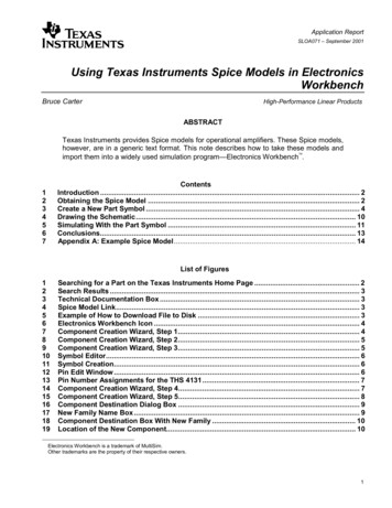
Parts BinInstrumentsSource components. Includes dependentand independent sources and groundsBasic components. Resistors, capacitors,inductors and variationsDiodes. Includes LED's and bridgenetworksBipolar and MOS transistorsMultimeter. Amps, volts, or Ohms.Function generator. Sine, square, andtriangular waveformsWattmeter.Oscilloscope (2-Channel)Analog components. Includes op ampsand other amplifiersTTL. A wide selection of 74 and 74LSpackagesCMOS. 4xxx and 74HC componentsBode plotter. Does both magnitude andphaseLogic AnalyzerMiscellaneous digital including VHDLand VerilogMixed analog/digital including convertersand 555 timerIndicators. voltmeter and ammeter,indicator lamps, and displaysMiscellaneous components including avacuum tube and a motorControl system components such assummers, multipliers, etc.RF componentsComponent mode button. Click this to addcomponentsComponent editor to modify componentparameters.Instruments. Click this to add an instrument.Electromechanical including a coil,transformer, and a relay.Report. Click this to generate a report.Mode and SimulationSimulate button. Alternatively, push F5 totoggle start/stop and F6 to pause.Analysis. Transient, AC, DC, and Fourierincluded.VHDL and Verilog simulation.Figure 2The principle icons on the three main tool bars of Workbench.
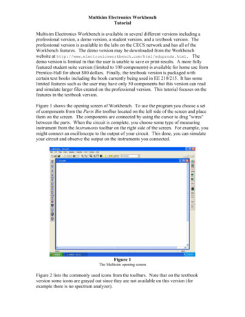
Example 1A simple resistor networkThe circuit which we will simulate has a dependent voltage controlled current source,four resistors, a battery, and a meter to measure the output. The finished circuit is shownin Figure 41.0kohmFigure E1-1A resistor network with a dependent current source.To begin click on the Source Components icon on the Parts Bin tool bar. This produces aselection of parts including various sources. Select a battery source from the menu byclicking on it. Click once more on the blank screen to place the battery. Figure E2 showsthe result.Figure E1-2Select a battery voltage source and place it on the blank screen.After placing the battery on the screen, double click on it to get a menu to set the batteryvalues. Change the battery value to 10 volts.
With the battery in place the next item to chose will be the voltage dependent currentsource. Choose this from the Source Components in the Parts Bin. A voltage dependentcurrent source has a value in mhos or amps/volt. Set this value to 0.001 mhos. Thecircuit also has a ground on either side of the dependent source. Select a ground symbolfrom the Source Components and place them on the diagram. Your circuit should looksomething like that shown in Figure E3.There are four resistors to be added to the circuit and we are done with the sources menu.You can close the source menu and open the Basic Components menu on the Parts Bintool bar. Note that there are two types of resistors in the parts bin. One type is a "realworld" resistor that has a value that you can purchase. The second type is a "virtual"resistor that is idealized and can have any value you choose to assign to it. Choose a1KΩ resistor and place it on the circuit diagram between the battery and dependentsource. Similary choose a 2KΩ resistor and place it immediately to the left of thedependent source. You can rotate a resistor by right clicking on it and choosing one ofthe rotation options. Choose another 1KΩ and 2KΩ resistor and place them to the rightof the dependent source. Rotate the resistors as needed so that your circuit looks like thatshown in Figure E4.Figure E1-3A battery and a voltage dependent current source have been placed.
Figure E1-4The circuit with all of the components in place. Note that resistors can be rotated by right clicking on themand choosing one of the rotation options.With the components in place you are ready to connect the wires. Workbench has nowire mode. You connect wires by moving the cursor to a component wire end, click onit, go to a second component and click on its wire end. Workbench will then fill in a wirebetween those two components. If you get a wire wrong, simply click on the wire andpush delete to get rid of it.It may be tempting to place components close enough together so that their terminalstouch and thereby avoid having to connect them together with a wire. But this doesn'twork in Workbench. Components must be connected together by wires.On occasion you may want to connect the end of one wire to a component. You cannotbegin a new wire from an old one unless you place a junction on the wire first. You cando this from the Place menu at the top of the screen.Sometimes Workbench does not choose a very good path between two points and thewire makes the circuit appear cluttered or unnecessarily complicated or the wire pathpasses through text. You can choose the path for any wire by clicking on intermediatepoints on the screen to form corners or junctions. You do this by first clicking on acomponent wire end, clicking on one or more intermediate points, and finally clicking onthe component wire end of the second component. The wire path will then go from thefirst component through each intermediate point to the second component. Afterconnecting the wires in the example your circuit should look like that shown in mR31.0kohmFigure E1-5The complete circuit with all of the components and wires in place.
The circuit in this example is ready for simulation except that we have no way to see theoutput. The simulator in Workbench outputs only to instruments which you connect tothe circuit diagram. For this dc example we will connect a voltmeter across R3 which wewill take as the output. The connect the voltmeter, select the multimeter from theInstruments toolbar on the right side of the screen. Place the multimeter near the R3resistor and connect the plus terminal to the top of R3 and the minus terminal to thebottom of R3 as shown in Figure E6. Double click on the multimeter and verify that it isset up as a dc voltmeter. Let the multimeter set up screen open so that you can view theresults of the simulation.Figure E1-6Connect a multimeter across R3. The voltage across R3 is taken as the output voltage. Double click on themultimeter to open the meter's setup and view screen.You can start the simulation by pushing the F5 function key, by pressing the on/offswitch at the top right corner of the Workbench screen, or by selecting run from theSimulation menu at the top of the screen. The result of the simulation will be shown onthe multimeter.Figure E7The multimeter showing the results of the simulation.The Multimeter also allow can be used as an ammeter or an ohmmeter and, by clickingon the Set. button you can manually set the impedance of the meters to conform to realworld instruments.Workbench also has a voltmeter and an ammeter in the Indicators section of the PartsBin.
Example 2An RC network using the oscilloscope and Bode plotterIn this example we use the oscilloscope and the Bode plotter in an RC circuit that has anAC source. The circuit which we will construct is shown in Figure E2-1.Figure E2-1The complete circuit showing the oscilloscope and Bode plotter.Begin by placing a 10KΩ resistor, a 1.0uF capacitor, a 100Ω resistor, an AC voltagesource, and an analog ground as shown in Figure E2-2. Use the cursor to draw in theconnecting wires. If you are unfamiliar with placing components and connecting wiresrefer to Example 1.R110kohmV1C110V 1000Hz 0Deg1.0uFR2100ohmFigure E2-2The basic RC circuit with all components in place. Note that you will have to change thedefault value of the AC voltage source to 10 Volts by double clicking on the source andsetting the value on the pop-up menu.For this circuit we will take the input to be the 10 volt AC source and the output to be thevoltage across the series combination of C1 and R2. Select the oscilloscope from theInstruments toolbar and connect the A channel to the top of V1 and the B channel to thetop of C1. It's not necessary to connect the oscilloscope ground. Your circuit shouldlook like that shown in Figure E2-3. Double click on the oscilloscope to open theoscilloscope control window and set the values as shown in the figure.
Figure E2-3The circuit with the oscilloscope connected. The time base is set to 200µsec/div. Setchannel A to 10 V/Div and channel B to 200 mv/Div. Set the y-position of channel A to 1.4 volts and the y-position of channel B to -1.6 volts.Push the F5 function key to run the simulation (or push the rocker switch at the top rightof the Workbench screen). The oscilloscope display will look like that shown in FigureE2-4.Figure E2-4The oscilloscope showing the simulation.The oscilloscope display has two arrows in red and blue near the top of the display. Usethe cursor to move the red arrow to a peak of the channel A display and move the bluearrow to the peak in the channel B display. The display will then show the difference intime as T2-T1 about equal to 160 µsec. Note that the input voltage source is at 1KHz sothe phase shift between the two is (160/1000)x360o 57.6o.Note that the oscilloscope has a Save button. This allows you to save the data collectedand displayed by the scope into an ascii file. The file can then be read by other programsuch as Matlab or Excel for reports or graphs. When you click on Save, you are
prompted to enter a file name which has the extension .scp by default. For this examplethe first few lines of such a file look like that shown in Figure E2-5 when read by aprogram like Notepad.Oscilloscope data forTime base: 0.000200 seconds per divisionTime offset: 0.000000 secondsChannel A sensitivity : 10.000000 volts per divisionChannel A offset: 14.000000 voltsChannel B sensitivity : 0.200000 volts per divisionChannel B offset: -0.320000 voltsChannel A connected: yesChannel B connected: yesColumn 1Column 2Column 3Time (S)Channel A Voltage(V)Channel B Voltage(V)TimeChannel AChannel 00000000e 000 0.0000e 000 -5.0931e-0027.294321988385e-006 4.5819e-001 -4.6255e-0021.729432198838e-005 1.0845e 000 -3.9247e-0022.729432198838e-005 1.7066e 000 -3.1671e-0023.729432198838e-005 2.3219e 000 -2.3557e-0024.729432198838e-005 2.9281e 000 -1.4938e-0025.729432198838e-005 3.5227e 000 -5.8467e-003.Figure E2-5This is the first part of a file containing the oscilloscope data. The data is in ascii formatand may be read by other program such as Excel.The file can be read into Excel directly and the column data can be plotted using theExcel plot features. To read the program into Matlab you must first strip off the headerdata so that the file consists only of the time base, Channel A, and Channel B data. Youcan then load and plot the three columns of data into a single Matlab variable with aMatLab statement such ass load('RCBode.txt'); %RCBode.txt is the amended scope file name.plot(s);Note that when plotting data in either Matlab or Excel the scaling that is done by theoscilloscope is lost.The Bode plotter is an instrument that allows you to look at the frequency response ofyour circuit. Select the Bode plotter from the Instruments tool bar on the right side of thescreen. The Bode plotter has both input and output terminals and has the additionalrequirement that your circuit must have at least one AC source as a circuit element. Forour example connect the input terminals of the Bode plotter directly across the AC sourceand the output terminals across the series combination of C1 and R2. This is shown inFigure E2-1 where a ground is used as a common connection.In use, the Bode plotter disables the AC source so that it has no real effect on the Bodeplot. The plotter applies a series of sinusoids to the input and monitors the sinusoids onthe output to determine the gain and the phase shift produced by the circuit.
Double click on the Bode plotter to get the control and output screen for the instrument.By tradition, a Bode plot is logarithmic plot of gain magnitude and phase vs. frequency.On Workbench you can alter the vertical and horizontal scales to be either linear orlogarithmic. For this example we will leave the traditional log plot in place. Change thehorizontal frequency scale so that the starting frequency (in window marked I) is at 10Hzand the ending frequency (in the window marked F) is at 100KHz. Run the simulation toget the Bode plot similar to that shown in Figure E2-6 below.Figure E2-6The Bode plot simulation showing the magnitude function. Note that you can move thered arrow horizontally and read out values in the window. The window above shows thatthe gain is at -20.442DB at a frequency of 165.059Hz.Click on the Phase button to see the phase curve. If you move the horizontal arrow to1000Hz you will see the display shown in Figure E2-7.Figure E2-7The phase curve with the marker set to about 1KHz. The phase is -55.207o which agreeswith the phase measurement taken on the oscilloscope.Like the oscilloscope, the Bode plotter also has a Save option which allows you to savethe data taken by the plotter as an ascii file. The first part of the Bode data file is shownin Figure E2-8. You can read the data file directly into Excel and make a prettier plot oryou can strip off the header information and read the data into Matlab.
Bode data forcolumn 1column 2column 3column 4trace name:Frequency (Hz)Gain (dB)Gain (Linear)Phase (Deg)Bode ResultFrequencyGain -----------------1.00000e 001 -1.46954e 000 8.44351e-001 -3.20393e 0011.02329e 001 -1.52790e 000 8.38697e-001 -3.26306e 0011.04713e 001 -1.58818e 000 8.32897e-001 -3.32275e 0011.07152e 001 -1.65042e 000 8.26950e-001 -3.38295e 0011.09648e 001 -1.71465e 000 8.20857e-001 -3.44365e 0011.12202e 001 -1.78090e 000 8.14620e-001 -3.50483e 0011.14815e 001 -1.84921e 000 8.08239e-001 -3.56645e 0011.17490e 001 -1.91960e 000 8.01715e-001 -3.62850e 0011.20226e 001 -1.99211e 000 7.95050e-001 -3.69093e 0011.23027e 001 -2.06676e 000 7.88246e-001 -3.75374e 001.Figure E2-8The first portion of the text file created by the Bode plotter. Click on the Save button tocreate this file.To get the Matlab plot, open the Bode plot data file in a word processor such as Word orNotepad, strip off all of the information above the raw data appearing in the 4 columns,and save the resulting file in a txt format. In Matlab you can plot the magnitude datausing the following commands:s load('BodeData.txt');semilogx(s(:,1),s(:,2));
Example 3Transient and AC AnalysisFor this example we will look at the analysis options under the simulate menu. Begin byconstructing the circuit shown in Figure E3-1.Figure E3-1An RC circuit with a Bode plotter and an AC source for use in doing the analysis options.Note that in this circuit we have changed the AC voltage source from the default 10 voltsto 1 volt. You might be tempted to use the function generator in place of the AC voltagesource but the function generator will not work with AC Analysis. Workbench requiresat least one AC voltage source in the circuit. We have also numbered the nodes since it isnecessary to know the node numbers for the analysis. You can number the nodes in yourcircuit by choosing Options Preferences and checking the Show node names box. Theoutput node is number 3.Figure E3-2The Bode plotter set up and result.Double click on the Bode plotter and set the frequency range to run from 100Hz to1MHz. (Note that in the Bode plot set up mHz stands for milli-Hertz and MHz stands forMegaHertz.) Run the simulation by pushing F5 and you will get he Bode plot shown inFigure E3-2.AC AnalysisThe first analysis that we will run on this circuit will be an AC analysis. From the menuselect Simulate Analysis AC Analysis. This will give you a menu screen similar tothat shown in Figure E3-3. Choose the starting and ending frequency range to run from100Hz to 1MHz and set the sweep type to linear with 100 points and a logarithmicvertical scale.
Figure E3-3Choose Simulate Analysis AC Analysis and set up the frequency parameters as shown.Next choose the Output variables tab from the top of the menu, select node 3 from the leftside of the page and click on the arrow to move it to the right side.Figure E3-4The output variables screen for AC Analysis. Select node from the left and click on the"Plot during simulation" button to move it to the right.Click on Simulate to complete the AC Analysis simulation. The results will appear in anew window called "Analysis Graphs" as shown in Figure E3-5. Note that the Bode plotwhich we did before also appears in this window under its own tab. The AC analysis andthe Bode plot both show the same information but they are plotted with different scales.The Bode plot has a logarithmic frequency scale and we chose a linear frequency scalefor the AC analysis.
Figure E3-5The AC Analysis. Note that this graph provides the same information as does the Bodeplotter but the scales are different.Transient AnalysisIn some books the term "Transient Analysis" refers to the step and impulse response of agiven circuit. For Workbench the term simply means the analysis of the circuit beginningat time 0 and running for a user specified time. The input is not limited to a step orimpulse.To do a transient analysis choose Simulate Analysis Transient from the menu. Thiswill produce an options screen similar to that shown in Figure E3-6. Change the end time(TSTOP) to 0.01 seconds. Click on the Output variables tab and verify that node 3 is theoutput variable. Click on the simulate button to get the results of the simulation. This isshown in Figure E3-7. Since we have an AC source as the input the transient analysisshows the sinusoidal start up at the output. The transient start up rapidly dies awaywithin a couple of cycles and settles to the steady state response of the circuit.To get a step response we would need to change the input voltage source to a PulseVoltage Source and set the frequency and duty cycle such that the circuit settles outduring each cycle. For this particular example, delete the AC Voltage source by clickingon it one time and pushing delete. Select a Pulse Voltage Source from the Parts Bin andconnect it in place of the AC source. Double click on the pulse source and set the voltagepulse to go from 0 to 1 volt, set the delay time to 0, the rise and fall times to 1 nsec, andpulse width to 10 msec with a period of 20 msec. Choose simulate to see the resultsshown in Figure E3-8.
Figure E3-6The Transient Analysis menu options. Change the value of TSTOP to 0.01 seconds.Figure E3-7The transient analysis results showing the sinusoidal start up at time 0.Figure E3-8The step response of the circuit.
Example 4Combinational Logic – A 2 to 4 decoder with enableFor this example we will simulate a 2-line to 4-line decoder with mechanical switches asinput devices and LED's as out put displays. The decoder logic will be made from 74LSTTL parts. The completed circuit is shown in Figure E4-1.Figure E4-1A 2-line to 4-line decoder with an enable. The red LED's indicate the state of the output.Begin by placing the TTL parts on the diagram first. Select the TTL icon from the PartsBin and choose the 74LS series. The 3-input nand gates are of type 74LS10 and there arethree gates per package so you will need two packages. For the inverters use the 74LS04part which has 6 gates per package and will need only three gates. Note that you canrearrange the text that goes with each package to allow for a neater configuration. InFigure E4-1 I have moved the UXX package designations onto the gates themselves. Thepin numbers shown would be used if you were actually building this circuit but since thisis just a simulation example the pin numbers for an individual gate are of no importance.Be sure to right click on the two bottom most inverters and rotate each counterclockwise. Your circuit should look something like that shown in Figure E4-2.
Figure E4-2Place the 3-input together using two packages of 74LS10 type. Use one package of74LS04 type for the inverters. Right click on the bottom most inverters and rotate themcounter-clockwise.Next we place the LED's on the board. These are on the Diodes menu in the Parts Bin.You have a choice of several colors. I have rotated the LEDs clockwise and moved theirnames around to tighten the configuration. After placing the first LED you can copy itand paste it for the others or you can select another LED from the in use list at the topcenter of the Workbench page. Add in four 330Ω resistors as shown in Figure E4-3.Figure E4-3Place four LEDs and four 330Ω resistors on the board as show.Finally we need to add the switches and the power supplies. Workbench has switches intwo places. The switches we will use are located on the Basic menu and they are singlepole double throw (SPDT) switches. (There are some momentary contact switches on theElectromechanical menu also.) Add three of the switches to the circuit and flip eachhorizontally as shown in Figure E4-4. Add in the digital power supply in three places forconvenience.
Notice that each switch has a corresponding "key" parameter. This refers to the key onthe keyboard which activates the switch during simulation. Double click on any switchand you get a menu that allows you to change this key. Change the two bottom switchesto have keys of A and B and set the top most switch to have a key of space.Figure E4-4The circuit with all of the components in place. Note that the key parameter of the threeswitches has been set to space, A, and B.Connect the wires on the circuit so that your final circuit looks like that shown in FigureE4-1. Test your completed circuit by running the simulation (push F5). If all is correct,you should be able to activate the switches by pushing the space bar, the A, or the B keyson the keyboard. To get the LEDs to light the top switch will need to be in the groundposition (active low) to enable the circuit. With the top switch down you will be able tolight any LED by varying the two A and B switches to one of four differentconfigurations.Complete the project by adding some text to your circuit. Add text by selectingPlace Place Text from the menu. Click the cursor at the location on the screen whereyou want the text and enter the text by typing it in. After entering the text you canchange its color by right clicking on it and selecting a color from the menu. You can alsochange the text font by selecting Options Preferences Font and selecting a font fromthe menu.
Example 5Sequential Logic – D-Type and JK Flip FlopsFor this example we will simulate a circuit containing a D-Type and a JK flip-flop andmake use of the function generator as a clock driver. The final circuit is shown in FigureE5-1.Figure E5-1A D-Type and JK flip-flop.Begin by adding the two flip-flops to the diagram. These are both on the TTL XXLSseries menu in the Parts Bin. For both the 74LS74 and the 74LS76 there are twoindependent flip-flops per package so you choose just one section from each package.After placing the flip-flops, choose a function generator and an oscilloscope and placethem as shown in Figure E5-2.Figure E5-2In this diagram we have chosen one section from the 74LS74 and one section from the74LS76 flip flop packages. These are in the TTL Parts Bin. The function generator andthe oscilloscope are chosen from the Instruments menu on the right.This circuit is all digital. We will add three 5 volt Vcc power sources and three digitalgrounds to the circuit from the Sources menu in the Parts Bin. Connect the wiring to thediagram as shown in Figure E5-1. Be sure to connect the clear and preset terminals of theflip-flops to 5. Note that the center terminal of the function generator is grounded andthe negative terminal is not used. The function generator is specified as having anamplitude, a frequency, a duty cycle, and an offset. The output wave is assumed to becentered vertically around 0 so that, for a square wave, an amplitude setting of 2.5 voltsand offset setting of 2.5 volts produces a 5 volt square wave that goes from 0 volts to 5volts. The negative terminal of the function generator puts out a signal of the oppositepolarity and is not used in this simulation. Set up the function generator and the
oscilloscope to look like those shown in Figure E5-3. (Double click on the functiongenerator or the oscilloscope to get the set up screens.)Figure E5-3Set up the function generator and the oscilloscope as shown above.Click on the simulate button in the top right corner or push function key F5. Thesimulation shows the JK flip-flop running at one half of the clock frequency.Figure E5-4A simulation of the flip-flop circuit.
Example 6Displays, Probes, Buzzers, and BussesFor this example we will simulate a circuit containing several indicators to illustrate howthey are used and we will add a bus to the system to simplify the wiring. We will firstsimulate the system without a bus as shown in Figure E6-1.Figure E6-1This circuit uses a decade counter to illustrate the use of displays, probes, and buzzers.For this circuit we need two TTL LS components which are the 74LS190 decadecounter and one section of a 74LS04 inverter. Select these items from the PartsBin and place them on the blank screen. Add a Clock Source from the Sourcesmenu of the parts bin and set its frequency to 120Hz and its voltage to 5volts.You will also need a 5 Volt Vcc source and two digital grounds. Your circuitshould look like that shown in Figure E6-2.Figure E6-2The TTL components and the sources have been added.Add the three indicators as the next items. Click on the indicators icon on theParts Bin and select the Hex Display item and select the part named DCD HEX.(All of the displays are somewhat idealized. The hex display shows a sevensegment hex number that corresponds to the logic level on its four input pins. Nopower supply is necessary. Likewise the other two displays have no power
connection and light up when the input terminals are activated.) Place the hexdisplay on the screen. Select a Buzzer from the same indicator menu and place iton the screen. Double click on the buzzer to set its voltage trip level. Set thisvoltage to 3 volts. You can also set a current level but we won't use that featurefor this example. Click on the red probe and place four of these on the circuitdiagram. Each of these has a trip point for being on or off which defaults to 2.5volts.Connect the wires to your circuit and get a final circuit similar to that shown inFigure E6-1.Note that for the hex display the least significant bit is pin 1 and the mostsignificant bit is pin 4. For the 74LS190 counter the least significant bit is pin 3and the most significant bit is pin 7. You might be tempted to flip the hex displayhorizontally by right clicking on it and selecting "flip horizontal" since this wouldplace the least significant bit closer to that of the counter's least significant bit andresult in less wire crossover. But if you do this with the display, Workbench alsoflips the display so the numbers displayed will appear as if you were looking at itfrom behind.For a real circuit it's unlikely that you will have a circuit like this connected to a120Hz clock source. If you did things would change so fast that you would beunable to see them. But if you slow the clock down to a reasonable rate such as10Hz the simulation takes a very long time.Simulate your finished circuit and verify that it does count upward from 0 to 9,that the probes do indicate the binary state of the output lines, and that the buzzeractually buzzes when the counter rolls over from 9 back to 0.Adding a BusBefore you add a bus to the system you will need to rearrange the hex display andthe probes and delete the wires which the bus will replace. Rearrange your circuitto look something like that shown in Figure E6-3. To add the bus, click onPlace Place Bus from the menu at the top of the screen. Adding the bus is likeadding a wire. Click on the starting point and click on first corner and doubleclick at the end point. The bus will be drawn to be a series of lines between yourclicks. If you double click on the comple
Multisim Electronics Workbench is available in several different versions including a professional version, a demo version, a student version, and a textbook version. The professional version is available in the labs on the CECS network and has all of the Workbench features. The demo version may be downloaded from the Workbench