Transcription
CFD Prediction of Cooling Tower DriftPrepared byRobert N. Meroney, Emeritus ProfessorWind Engineering and Fluids LaboratoryCivil Engineering DepartmentColorado State UniversityFort Collins, CO 80525October 25, 2004Revised August 5, 2005ABSTRACT:Drift of small water droplets from mechanical and natural draft cooling tower installations can contain watertreatment chemicals such that contact with plants, building surfaces and human activity can be hazardous.Prediction of drift deposition is generally provided by analytic models such as the US Environmental ProtectionAgency approved ISCST3 (Industrial Source Complex Short Term Version 3) or SACTI (Seasonal-Annual CoolingTower Impact) codes; however, these codes are less suitable when cooling towers are located midst taller structuresand buildings. A computational fluid dynamics code including Lagrangian prediction of the gravity driven butstochastic trajectory descent of droplets is considered and compared to data from the 1977 Chalk Point Dye TracerExperiment. The CFD (computational fluid dynamics) program predicts plume rise, surface concentrations, plumecenterline concentrations and surface drift deposition within the bounds of field experimental accuracy.KEYWORDS:Drift, Deposition, Cooling Tower, Computational Fluid Dynamics1
1.0INTRODUCTIONMechanical and natural draft cooling towers are routinely used to condition air and water for power plants and airconditioning systems. Water droplets become entrained in the air stream as it passes through the tower. When asmall amount of circulating water in a cooling tower is entrained and carried aloft by the air stream in the form ofdroplets, which vary from a few to several thousand microns in diameter, the droplets are referred to as drift. Whileeliminators strip most of this water from the discharge stream a certain amount discharges from the tower as drift.The rate of drift loss is a function of tower configuration, eliminator design, airflow rate through the tower and waterloading. Because such drift contains the minerals of the makeup water and often contains water treatment chemicals,contact of these chemicals with plants, building surfaces and human activity can be hazardous (U.S. EPA, 1984,1989).Cooling tower drift includes larger droplets, which fall out of the often-visible fog plume due to the effect of theearth’s gravitational field. The rate of descent of the fluid droplets depends upon a balance between theaerodynamic drag force and the gravitational force exerted by the earth on the individual droplet. Sedimentation ofsuch droplets downwind of the cooling towers may result in an increase in ground level concentrations of coolingtower water treatment chemicals. The ground can then retain the chemicals by processes such as impaction andabsorption. The transport and dispersion of gases and fine aerosols from the cooling tower exits can be predicted byanalytic programs (such as the Industrial Source Complex (ISC3) or the Seasonal/Annual Cooling Tower Impact(SACTI) models) or when significant building interactions are present by physical modeling in environmental windtunnels. (See Sections 2.1.2 and 2.1.3 for references)Analytic models such as the ISC3 group include plume rise formulae and adjustments for building downwash,buoyant/dense plume behavior, gravitational settling and wet/dry deposition. These formulae include corrections forbuilding downwash by Huber & Snyder (1982) or Scire & Schulman (1980) based on physical modelingmeasurements in environmental wind tunnels. The corrections for gravitational settling are calculated fromestimates of fall velocity of individual droplets based on physical modeling measurements of drag coefficients forsmall particles in laboratory facilities. SACTI and some CFD codes (e.g. FLUENT) also include thermodynamiceffects due to phase changes (condensation and evaporation) which can affect plume and drift behavior.Unfortunately, neither of these analytical approaches includes the influence of nearby large buildings on the flowfields, which affect the local building downwash and cooling tower drift. Although the background flow fields andgaseous plume motions can be accurately simulated by physical modeling in environmental wind tunnels atmoderate velocities, the correct scaling of droplet and particle drift requires that the simulations be run at extremelylow facility velocities, which then distorts the model flow fields (Kennedy and Fordyce, 1974; Jain and Kennedy,1978). A third approach to estimate drift and droplet deposition which includes the effects of ambient winds,2
building wakes, exhaust jets and surrounding buildings and terrain is that of computational fluid dynamics (CFD),i.e. solving the relevant equations of motion by numerical means. This method is primarily limited bycomputational resources and the accuracy of turbulent models (McAlpine and Ruby, 2004).This paper discusses the status of computational and hybrid modeling of wind engineering situations in Sections 1.1and 1.2. Then it reviews existing analytic methods to predict drift in Section 2.1, considers the sensitivity of inputconditions during drift predictions in Section 2.2, and examines the methodology used in a typical commercial code,FLUENT, to predict drift in Section 2.3. Section 3.0 compares CFD calculations of drift during the 1977 ChalkPoint cooling tower experiments to observations and analytic predictions. Section 4.0 summarizes the results ofthese considerations and calculations.1.1Computational ModelingNumerical modeling, despite its many limitations associated with grid resolution, choice of turbulence model, orassignment of boundary conditions is not intrinsically limited by similitude or scale constraints. Thus, in principle,it should be possible to numerically simulate all aspects of plume transport, dispersion, and/or drift. In addition itshould be possible to examine all interactions of plume properties individually, sequentially and combined toevaluate nonlinear effects (Murakami, 1999; Stathopoulos, 1999). It is this tremendous potential that has led windengineering practitioners to more frequently present results of such numerical studies in professional and tradejournals and promotional materials. Realistically, however, the choice of domain resolution, turbulence models, andboundary conditions constrain predictions.Hence, continued verification and validation is required at almost every level of CFD prediction (Castro andGraham, 1999; Castro, 2003; Slater, 2004).1 Various criteria for measuring agreement between predictions and fullor model-scale measurements are available including scatter diagrams, classical ANOVA (Analysis of Variance),pattern comparison tests and weighted average fractional bias plots (Shin et al., 1989, 1991). Several organizationshave established committees and groups to focus on the quality of and trust in CFD applied to practical applications(e.g. QNET-CFD, 2004; NPARC Alliance, 2004; ERCOFTAC, 2000; AIAA, 1998).1Verification is defined as the process of determining that a model implementation accurately represents thedeveloper’s conceptual description of the model and the solution to the model. Or: Procedure to ensure that theprogram solves the equations correctly. Validation is defined as the process of determining the degree to which amodel is an accurate representation of the real world from the perspective of the intended uses of the model. Or:3
1.2Hybrid ModelingA “hybrid” model is one that results from the union of concepts or results from two unrelated methodologies (eg.experimental and numerical). Hangan (2004) suggested one call the hybrid approach, the C-FD-E concept. The CFD-E concept considers the interplay between computational fluid dynamics (CFD) and experimental fluiddynamics (EFD). Hangan argues that the two tools have to play complementary rather than opposed roles in thefurther development of fluid dynamics. There are several reasons why hybrid or joint fluid/computational modelingshould be useful for evaluating the validity of dispersion models and even directly predicting the behavior ofdispersion during diffusion incidents: theoretical, dispersion comparability, controlled conditions and expense. Thevery use of the word “hybrid” implies a combination of initially unrelated concepts of heterogeneous origin thatresults in an offspring that has hopefully the best qualities of both parents. Indeed, such crossbreeding often resultsin ‘hybrid vigor’ that has even better and stronger characteristics than either parent. For example, Both methods permit the individual control of many variables which permits the analyst to isolate drivingor dominant transport mechanisms, Fluid modeling can provide data in situations where the actual physical mixing mechanisms are vague,confused or obscured by other phenomena, Computational modeling can provide data at greater spatial resolution than is practicable during fluidmodeling due to instrumentation, time or cost limitations, and Dispersion in fluid modeling situations incorporates mixing at all time scales, whereas time dependentsolutions in CFD often require the dedication of massive computational resources. Computational modeling can be employed to explore further into the parametric space of a problem.When used together the analyst is able to confidently assess model reliability, model generality, and modelrobustness. Indeed engineering groups are often reluctant to make critical design decisions based solely on CFD,instead acquiring similar data from independent sources, such as wind tunnel testing that mitigates the perceivedrisks due to feared deficiencies in CFD data. Viegas remarked during the 1993 NATO Advanced Study Institute onWind Climates in Cities that “numerical and experimental methods are complementary, the ideal situation being thatboth of them are carried out in parallel.” (Cermak et al., 1995)2.0ANALYTIC AND COMPUTATIONAL PREDICTION OF COOLING TOWER DRIFTEstimation of the impact of cooling tower drift on downwind deposition of droplet born toxins in the presence ofbuildings can be difficult. Initial interest in drift was associated with dispersion of radioactive particles from nuclearaccidents or nuclear power plant sites (Pasquill, 1962; Van der Hoven, 1968). Later the impact of accumulated saltson downwind vegetation associated with large ocean-side fossil and nuclear power plants using salt-water orProcedure to test the extent to which the model accurately represents reality.4
brackish water in natural and mechanical draft cooling towers drove investigations into drift behavior (ASME,1975). A few field studies performed between 1965 and1984 examined cooling tower plume rise, visibility, anddownwind concentrations. Unfortunately, only a couple of these actually measured deposition rates downwind.2.1Analytic ModelsDespite limited field data, concern about drift and deposition led to more than a dozen separate analytic models topredict downwind ground-level concentrations and deposition rates. Chen (1977) and Chen and Hanna (1978)compared ten drift deposition models using a set of standard input conditions for a natural draft cooling tower. Theyconcluded most of the models agree within a factor of three; however, when all ten models are compared, thepredicted maximum drift deposition differs by two orders of magnitude, and the downwind locations of themaximum differ by one order of magnitude. These comparisons occurred before improved sets of field data fromthe Chalk Point Dye Tracer Experiments were available after 1977.Policastro et.al. (1978) compared most of the same drift deposition models to the new Chalk Point experimentaldata. They concluded, “None of the existing models performed well.” The authors observed that even for this “bestavailable” data the statistical significance of the data may be questionable considering only 10 to 50 droplets weretypically obtained on the sensitive measurement papers over a four-hour period.Policastro et al. (1981a, 1981b)developed the SACTI model specifically to improve drift prediction, yet they concluded for a model to predictwithin a factor of three of measured data can be considered successful prediction. (Success within a factor of threemeans the prediction is within the range encompassed by one-third and three times the measured value, but sampleswhere either the measured value is zero or the model prediction is zero are not counted.)Drift predictions are also quite sensitive to initial conditions. In order to determine how the variations in updraft airspeed, temperatures, and drift mass emission droplet spectra would affect drift transport modeling results, Webb etal. (1978) performed a sensitivity study using input data gathered during the Chalk Point Cooling Power Project in1976. They inserted these variations into the ESC/Schrecker drift model (still considered a model nearly on par withthe SACTI model). The standard deviations of test averages for tower exhaust velocity, tower updraft airtemperature, and emission rates varied by 13, 4.5, and 42 % respectively. Drift mass emission varied by factorsfrom 24 to 3 for droplet sizes at 1000 and 50 :m, respectively. Consequently, predicted deposition rates varied byfactors of 60, 15, 8 and 3 at 300, 500, 1,000 and 10,000 m, respectively. They concluded variations in the driftemission droplet spectrum have the greatest effect on model calculations of downwind mineral mass deposition.A review of available drift models suggest that currently the most frequently used for short range transport are theK.S. Rao modifications to the EPA Point, Area Line Source Algorithm (PAL2.1), the EPA Industrial Source5
Complex Short Distance 3 (ISCST3) model, and the Argonne National Laboratory Seasonal/Annual Cooling TowerImpact (SACTI) model. These are considered in detail below.2.1.1PAL2.1 Model: This model was undertaken to develop concentration algorithms for the EPA PollutionEpisodic Model (PEM) in the early 1980s (Petersen and Rumsey, 1987). The analytical plume model predictsatmospheric transport, diffusion, deposition, and first-order chemical transformation of gaseous and particulatepollutants. It treats gravitational settling and dry deposition from elevated sources by solving the equations ofmotion based on gradient transfer or K-theory (Rao, 1981, 1983). The model’s strength is its simplicity and ease ofuse. Unfortunately, its greatest disadvantages are also its simplicity since it does not adjust for complex buildingenvironments where separation, reattachment and recirculation of the flow field can occur. It is not a true ballistictrajectory model; hence, it is less likely to predict the behavior of large droplets near (within 1-2 km) of the sourcewell. This model is also described briefly by Hanna, Briggs and Hosker (1982) in their well-known Handbook ofAtmospheric Diffusion. This model has not been used extensively recently, but it is included here due to itshistorical significance, and its analytic rigor.2.1.2ISCST3 Model:The most widely used air quality model is the U.S. Environmental Protection Agency’sIndustrial Source Complex Short Term Model 3 (ISCST3). This model is used to address the air quality impactsfrom stationary sources to demonstrate compliance to permitting regulations. While the model is useful forestimating pollutant concentrations beyond the zone of building wakes it is not intended for analysis within arecirculation zone nor can it account for air movement deflections and turbulence caused by obstructions downwindfrom the source complex.The ISCST3 model provides options to model emissions from a wide range of sources that might be present at atypical industrial source complex. The basis of the model is the straight-line, steady-state Gaussian plume equation,which is used with some modifications to model simple point source emissions from stacks, emissions thatexperience the effect of aerodynamic downwash due to nearby buildings, isolated vents, multiple vents, etc. (U.S.EPA, 1995b). Emissions are categorized into four types, i.e., point sources, volume sources, area sources, and openpit sources. The model accepts hourly meteorological data records to define the conditions for plume rise, transport,diffusion and deposition.Plume rise caused by momentum or buoyant forces are accounted for by adjusting thesource height and plume trajectory. Thermodynamic effects on plume behavior, specifically latent heat effects dueto condensation or evaporation of water vapor or drifting particles are not included. Seasonal or annualconcentrations are calculated by weighting downwind results for time dependent variations in source strength, windfields, wind directions and climatic stability.Particles (or droplets) included with the emissions are brought to the surface through the combined processes ofturbulent diffusion and gravitational settling. Once near the surface, they may be removed from the atmosphere and6
deposited on the surface. The removal is modeled in terms of deposition velocity (vd), by assuming the depositionflux of material to the surface is equal to the product vd Pd , where Pd is the airborne concentration just above thesurface. Such deposition reduces the concentration of particulates within the plume, and thereby alters the verticaldistribution of the remaining particulates. A corrected source-depletion model developed by Horst (1983) is used toobtain a vertical term that incorporates both the gravitational settling of the plume and the removal of plume mass atthe surface. These effects are incorporated as modifications to the Gaussian plume equation. Gravitational settlingis assumed to result in a “tilted plume”, so the effective plume height of the release constantly decreases at a rateproportional to droplet settling velocity, vg . Then local ground level concentrations are adjusted by a “sourcedepletion factor” that can be considered a ratio of the current mass emission rate to the original mass emission rate,and the remaining source mass is also redistributed in the vertical to account for the mass adjustment.The adjustment factors depend on the size and density of the particles being modeled because they affect the totaldeposition velocity; hence, for a given source of particulates, ISCST3 allows multiple particle-size categories to bedefined. The final deposition at the wall then becomes the sum of the terms for each particle-size category, weighted2by the respective mass-fractions.2.1.3SACTI Model: Staff at the Argonne National Laboratory working for the Electric Power Research Institutedeveloped this model to predict plume and drift behavior from multiple tower and cell configurations of natural andmechanical draft cooling towers (Policastro et al., 1981a, 1981b). The SACTI Model incorporates a number ofsignificant improvements over previous analytic models. These include i) use of an advanced integral model forcooling tower plume trajectory and dispersion (Schatzmann and Policastro, 1984), ii) incorporation of improveddroplet evaporation models which include adjustments for ambient temperatures, humidity and the effects of3dissolved solids, iii) the choice of up to five “breakaway models” for when the droplets leave the cooling towerplume and enters ambient air, and iv) the use of ballistic trajectory calculations to determine behavior of individualdroplets as they change droplet diameter and move from within the plume to ambient air with associated changes inair speed and drag. The model does include empirical corrections for the effects of tower downwash on the grossplume motions through a modification of the entrainment function; however, it does not include corrections for theinfluence of upwind or downwind buildings or terrain.The behavior of the single plume SACTI Model was validated against the Chalk Point Dye Tracer Study (Policastroet al., 1978b, 1981a). The behavior of the multiple plumes SACTI Model was validated against the multiple unitmechanical draft cooling towers at Pittsburgh CA (Policastro et al., 1981b). They concluded a model that could2Another EPA promoted program which includes deposition based on droplet size and gravitational settling is themodel CALPUFF (U.S. EPA, 2003). This model is primarily recommended for long range transport (distances 50km), but includes similar physics for calculating particle movement and deposition as ISCST-3.3SACTI is the only analytic model which properly accounts for phase changes and latent heat effects.7
predict deposition within factors of 3 should be considered sufficiently accurate given the uncertainties inmeteorology, cooling tower performance, and model assumptions. Comparisons were presented for sodiumdeposition flux, drop number flux, average diameter, and liquid mass deposition flux.The Chalk Point facility included two large natural draft cooling towers located in flat tide-water terrain on theChesapeake Bay, MD. Data were limited to moderate-to-large wind speed, high ambient relative humidity, andstrongly stable ambient stratification. Hence, only a minimal effect of droplet evaporation and ambient turbulenceeffects were examined. Deposition of Rhodamine-WT fluorescent dye tracer was measured only at 500 and 1000 mdownwind of the cooling tower. The fallout of larger droplet diameters will dominate deposition at these shortdistances. For the Chalk Point comparisons they concluded that, given the “correct” choice of breakaway criterion,agreement occurred with only one failure over the entire measured data set, and they asserted the SACTI model wasas good as or better than other drift models.The Pittsburgh facility consisted of seven oil-fired units. Units 1-6 employed once-through cooling, while Unit 7 iscooled by two 13-cell rectangular mechanical draft cooling towers located 0.5 km from the unit. The towers werestated by the manufacturers to have a guaranteed drift rate of 0.004%, but leaks around the cooling tower drifteliminators allowed significantly higher drift emissions in some cases. Data were sampled along five arcs locatedbetween 120 to 750 m downwind of Tower Unit 7-1 and between 250 to 1000 m downwind of Tower Unit 7-2.Downwind deposition measurements were often coordinated with simultaneous source measurements. Eight fieldsurveys were conducted during June 1978. For model comparisons a single-composite drift droplet spectrum wasused independent of test date. For the Pittsburgh comparisons the authors concluded that the SACTI modelpredicted deposition within a factor of 3, 50% of the time.2.1.4 Model Limitations: These analytic models have assumptions which limit their application to near fieldtransport and diffusion. They are: Stack emission downwash adjustment presumes the source building and its stack is not in the recirculationregion of other buildings, The effect of streamline deflection on plume trajectories is not considered, The effect of the velocity deficit in the wake on plume rise is neglected; There is no accounting for plume material captured by the near wake on far wake concentrations, Stack plume height adjustment algorithms presume the building is a simple rectangular form withcharacteristic height, width and depth, Plume concentrations are not reliably predicted within the immediate recirculation region of the buildingwake, and8
The model does not account for the effect of any upwind or downwind buildings on plume trajectory orenhanced dispersion.In addition the PAL 2.1 and ISCST3 models are further constrained because: Gravitational settling algorithms used assume relevant particle sizes are small ( 0.1 mm); hence, the modeldoes not predict the behavior of large particles, Thermodynamic effects of condensation and evaporation on plume and drift behavior are not considered,and The programs do not adjust for the effect of the interaction of large nearby source jets (like multiple coolingtower units on a mechanical draft cooling tower) on plume rise and turbulent mixing.Some of these limitations have been addressed in the development of the ISC-PRIME and AERMOD-PRIMEmodels proposed to replace the ISC-3 series (Schulman, et al., 2000; Petersen, 2004); however, although PRIME canbe used with more than one building close to the source stacks, it cannot be used to compute the plume path throughor affected by the building cavities for another building or group of buildings at a distance downwind from the initialindustrial source complex (Ruby and McAlpine, 2004).2.2Droplet Particle Distributions at Cooling Tower ExitCooling tower drift consists of droplets from the cooling water stream, which are entrained out of the tower in theexhaust gas flow. In order to minimize drift emissions, modern cooling towers commonly employ drift eliminatorsystems. The magnitude of the drift loss is influenced by the number and size of droplets produced within thecooling tower. These are in turn determined by the fill design, air and water patterns (counter flow, cross flow, fanassisted, induced draft, etc.), type of drift eliminator installed, etc. (U.S. EPA, 1995; Moore et al., 1978).To reduce the drift from cooling towers, drift eliminators are usually incorporated into the tower design to remove asmany droplets as practical from the air stream before exiting the tower. The drift eliminators rely on inertialseparation caused by exhaust flow direction changes while passing through the eliminators. Types of drifteliminator configurations include herringbone (blade-type), waveform, and cellular (or honeycomb) designs. Drifteliminators are typically rated in terms of the percentage of recirculating cooling water flowing through the systemthat escapes the tower. Lower efficiency systems are those, which produce values between 0.008 to 0.02 percent,whereas higher efficiency systems claim performance levels of 0.008 percent. (U.S. EPA, 1989, 1995; Becker andBurdick, 1994)9
Many measurement techniques are used to measure droplet distributions. No single method enjoys universalacceptance as the best overall drift measurement technique. In the absence of comprehensive comparative analysisof the various measurement devices, it is difficult to make comparisons of data obtained with different equipment(Golay et. al., 1985). It is also possible that many of the methods used to measure droplet distributions are biasedtoward smaller particles (ASME, 1975; Chen and Hanna, 1977).Webb et al. (1978) concluded that predictions of drift deposition were most sensitive to the initial choice of dropletparticle distribution at the cooling tower exit. Schrecker (1978) noted that during the Chalk Point experiment some16 drift-droplet size distributions were measured over the tower’s exit plane on different days. The variability of themeasured data were large enough that his predictions by analytic models produced deposition rates at distances lessthan 1 km which varied by factors of 10 and at greater distances by factors of 3.Quite frequently measured droplet distributions are bimodal with peaks at small and medium or large dropletdiameters. It is likely that such distributions are associated with inadequacies in design or subsequent maintenanceof drift eliminators. Large droplets of the order of 1000 microns may be generated by i) gaps in the drift eliminatorscaused by cooling tower structural members, ii) variations in local air velocities due to fan or tower configurationoutside the drift eliminator design range, and iii) re-entrainment of collected drift occurring due to wateraccumulated on structural members, cooling tower fan blades, and the surface of the fan stack. Since these surfacesare downstream of the drift eliminators, the droplet size is determined by the entrainment process and local velocity(PGT, 2003). Indeed, emissions from such sources may comprise most of the mass of the drift emitted by coolingtowers. Consequently, the prediction of the size distribution of the drift for a cooling tower can be subject to greatuncertainty.Nonetheless, if deposition predictions are to be made, an informed selection of a “reasonable” droplet distribution isnecessary. A review of the literature produced nine sets of data for the cumulative mass fraction distributions ofdroplets (Lindahl, 2003 [typical Marley MDCT]; Hanna et al., 1978 or 1981 [Chalk Point NDCT (Natural DraftCooling Tower)]; ERT, 1978 [ Hat Creek MDCT (Mechanical Draft Cooling Tower)]; Policastro et al., 1981b[Pittsburgh CA MDCT]; Wilber and Vercauteren, 1986 [Palo Verde MDCT]; Chen and Hanna, 1978 [Idealizednormalized distribution]; Chen and Hanna, 1978 [Turkey Point MDCT]; Jallouk et al., 1975 [Oak Ridge NationalLaboratory MDCT]; and Wilstrom and Ovard, 1973 [Ecodyne MDCT].The cumulative mass fraction for these cases tended to decrease exponentially with increasing particle diameter;hence, the data were fit to a Rosin-Rammler particle distribution of the form:nCum Mass Fraction exp (-(d/dmean) ),10
where dmean is the mean particle diameter, and n is known as the shape factor. Comparisons resulted in the followingtable:Table 1: Mean Diameter and Shape Factor Parameters in Rosin-Rammler Cumulative Mass Fraction DistributionsData Setdmean (mm)nMarley MDCT0.091.00Chalk Point NDCT0.090.65Turkey Point MDCT0.071.20Hat Creek MDCT0.150.85Pittsburgh MDCT1.001.00Oak Ridge MDCT0.101.00Palo Verde MDCT0.451.75Chen & Hanna Idealized0.302.00Ecodyne MDCT1.800.85Data seems to fall into two categories with either d mean 0.1mm and n 1.0 or dmean 1.0 mm and n 1.0.Thesecond category reflects the presence of a significant number of large particles. In a private communicationPolicastro (2004) remarked that droplet distributions often had more large droplets than manufacturers like to admitdue to end losses, splash and condensation on the cooling tower structure with subsequent re-entrainment.2.3FLUENT CFD Model of Cooling Tower DriftAn alternative approach to estimate drift deposition is to use CFD (
Viegas remarked during the 1993 NATO Advanced Study Institute on Wind Climates in Cities that "numerical and experimental methods are complementary, the ideal situation being that . (Cermak et al., 1995) 2.0 ANALYTIC AND COMPUTATIONAL PREDICTION OF COOLING TOWER DRIFT Estimation of the impact of cooling tower drift on downwind deposition of .