Transcription
sensorsArticleA Hydraulic Pump Fault Diagnosis Method Based on theModified Ensemble Empirical Mode Decomposition andWavelet Kernel Extreme Learning Machine MethodsZhenbao Li 1,2 , Wanlu Jiang 1,2, *, Sheng Zhang 1,2 , Yu Sun 1,2 and Shuqing Zhang 3123* Citation: Li, Z.; Jiang, W.; Zhang, S.;Sun, Y.; Zhang, S. A Hydraulic PumpFault Diagnosis Method Based on theModified Ensemble Empirical ModeDecomposition and Wavelet KernelExtreme Learning Machine Methods.Sensors 2021, 21, 2599. https://doi.org/10.3390/s21082599Hebei Provincial Key Laboratory of Heavy Machinery Fluid Power Transmission and Control,Yanshan University, Qinhuangdao 066004, China; lizhenbao@stumail.ysu.edu.cn (Z.L.);zsqhd@ysu.edu.cn (S.Z.); zhang py@stumail.ysu.edu.cn (Y.S.)Key Laboratory of Advanced Forging & Stamping Technology and Science, Yanshan University,Ministry of Education of China, Qinhuangdao 066004, ChinaSchool of Electrical Engineering, Yanshan University, Qinhuangdao 066004, China; zhshq-yd@163.comCorrespondence: wljiang@ysu.edu.cnAbstract: To address the problem that the faults in axial piston pumps are complex and difficult toeffectively diagnose, an integrated hydraulic pump fault diagnosis method based on the modifiedensemble empirical mode decomposition (MEEMD), autoregressive (AR) spectrum energy, andwavelet kernel extreme learning machine (WKELM) methods is presented in this paper. First, thenon-linear and non-stationary hydraulic pump vibration signals are decomposed into several intrinsicmode function (IMF) components by the MEEMD method. Next, AR spectrum analysis is performedfor each IMF component, in order to extract the AR spectrum energy of each component as faultcharacteristics. Then, a hydraulic pump fault diagnosis model based on WKELM is built, in orderto extract the features and diagnose faults of hydraulic pump vibration signals, for which therecognition accuracy reached 100%. Finally, the fault diagnosis effect of the hydraulic pump faultdiagnosis method proposed in this paper is compared with BP neural network, support vectormachine (SVM), and extreme learning machine (ELM) methods. The hydraulic pump fault diagnosismethod presented in this paper can diagnose faults of single slipper wear, single slipper loosingand center spring wear type with 100% accuracy, and the fault diagnosis time is only 0.002 s. Theresults demonstrate that the integrated hydraulic pump fault diagnosis method based on MEEMD,AR spectrum, and WKELM methods has higher fault recognition accuracy and faster speed thanexisting alternatives.Academic Editor: Chris KarayannisReceived: 11 March 2021Accepted: 5 April 2021Keywords: hydraulic pump; fault diagnosis; modified ensemble empirical mode decomposition(MEEMD); wavelet kernel extreme learning machine (WKELM)Published: 7 April 2021Publisher’s Note: MDPI stays neutralwith regard to jurisdictional claims inpublished maps and institutional affiliations.Copyright: 2021 by the authors.Licensee MDPI, Basel, Switzerland.This article is an open access articledistributed under the terms andconditions of the Creative CommonsAttribution (CC BY) license (https://creativecommons.org/licenses/by/4.0/).1. IntroductionIn recent years, modern industrial equipment has developed in the direction of complexity, high speed, and intelligence. This not only ensures the quality of the products, butalso greatly reduces the associated production costs and significantly improves productionefficiency. However, in the actual production process, due to the continuous expansionof system scale and the increasing complexity of the structures involved, the probabilityof equipment failure has been gradually increasing. Therefore, it is very important toimprove the safety and reliability of such equipment. In this regard, it is necessary notonly to improve the reliability of the equipment in the process of equipment design andmanufacturing, but also to carry out real-time status monitoring and fault diagnosis duringthe operation of the equipment. In this way, we can detect the fault initially, then predictthe location and cause of the fault, in order to provide accurate information for predictivemaintenance. Therefore, more and more attention has been paid to fault diagnosis andprediction technology, for which a lot of research work has been carried out [1–4].Sensors 2021, 21, 2599. com/journal/sensors
Sensors 2021, 21, 25992 of 24Hydraulic systems have the advantages of small size, light weight, high power, smoothtransmission, and fast response. Hydraulic systems have been widely used in the aerospace,shipbuilding, metallurgical, machine tool, agricultural machinery, and engineering machinery industries, among other fields. The wide application of hydraulic systems hasgreatly promoted the development of industrial production [5]. Since entering the 21stcentury, hydraulic systems and hydraulic equipment have become more complicated andlarge-scale. Once a failure occurs, it not only can damage the equipment, but may evencause casualties [6]. Hydraulic pumps have the characteristics of complex structure, highspeed, high pressure, and continuous operations, and are the most prone to failure. Therefore, fault diagnosis technology for hydraulic systems has become a research hotspot inrecent years.In fault diagnosis, the first step is to extract fault features from the acquired data [7,8].Feature extraction is the process of obtaining fault features through signal processing [9,10].Considering that the vibration signal of a hydraulic pump has non-linear and non-stationarycharacteristics, it is difficult to extract the fault features accurately by using traditional timeand frequency-domain analyses. The key information of the hydraulic pump vibrationsignal can be extracted more accurately by using time-frequency characteristic analysismethods. Time-frequency analysis methods include non-adaptive analysis and adaptiveanalysis. Adaptive analysis refers to the modal decomposition and reconstruction of thesignal, according to the characteristics of the signal, in the process of signal processing, inorder to achieve good analysis results.Considering the mode mixing phenomenon of the empirical mode decomposition(EMD) method [11,12], Wu et al. proposed the ensemble empirical mode decomposition(EEMD) method, which effectively suppresses modal mixing by adding Gaussian whitenoise to the original signal [13]. In view of the shortcomings of the EEMD method, scholarshave carried out a lot of research. Finally, Zheng et al. proposed the modified ensembleempirical mode decomposition (MEEMD) method [14], which adds a pair of Gaussianwhite noises with the same amplitude and opposite signs, such that they cancel each otherand the influence of the noise on the signal is reduced. Compared with the EEMD method,this method has a better decomposition effect. Jiang et al. applied the MEEMD method tothe fault diagnosis of the main shaft bearing of a wind turbine [15]. Their method showedgood results, in terms of training accuracy and training speed, which verifies the feasibilityof this method. Zheng proposed a method combining MEEMD and generalized adaptive Stransform (AGST), which was successfully applied to the vibration signal analysis of aninternal combustion engine [16]. Shi et al. applied the MEEMD method to fault featureextraction of rolling bearings, which not only effectively suppressed the phenomenon ofmodal mixing but also greatly reduced the number of pseudo-components and accuratelyextracted the weak fault information of rolling bearings [17]. Although the MEEMDmethod has been widely used in the field of fault diagnosis, it has seldom been reported inhydraulic system fault diagnosis. Therefore, in this paper, we applied it to the vibrationsignal feature extraction of an axial piston pump, in order to improve the accuracy offault identification.In 2004, Professor Huang from Nanyang Technological University in Singapore proposed a new single-hidden layer feedforward neural network, called the extreme learningmachine (ELM) [18–20]. In 2018, Zhang et al. proposed a method combining evidencetheory and ELM, which effectively solved the classification problem of incomplete data [21].However, it should be noted that the optimal number of neurons in the hidden layer obtained by the incremental extreme learning machine and its improved method may be verylarge, thus wasting a lot of unnecessary training time.As the ELM method needs to set the number of hidden layer neurons and randomlyselect input weights and hidden layer biases, ELM instability is inevitable. Therefore,Huang et al. introduced a kernel function into the ELM to propose the kernel-ELM (KELM)method. This method avoids the problems of artificially setting the number of hiddenlayer neurons and randomly selecting the input weights and hidden layer biases in ELM
Sensors 2021, 21, 25993 of 24by means of kernel function mapping. KELM can achieve very high training accuracy byusing the powerful mapping ability of kernel function [22]. To date, KELM has been widelyused in various fields. One study [23] has proposed a parallel KELM, which effectivelyimproved the computing speed of KELM. Cho et al. applied a K-ELM to correctly classifythe stress levels to reflect five different levels of stress situations [24]. Zhang et al. proposeda soft sensing algorithm that can detect alumina concentration by the electrical signalssuch as voltages and currents of the anode rods [25]. Yang et al. combined the multiscale feature energy with the KELM to effectively diagnose the airflow jamming fault of afluidized bed [26]. Zhang et al. applied the KELM to the fault diagnosis of a coal mill andoptimized the kernel parameters with particle swarm optimization (PSO) [27]. Yang et al.proposed a deep kernel extreme learning machine (DK-ELM), which has been successfullyapplied to aero-engine fault diagnosis [28]. Considering that wavelet functions have theadvantages of time–frequency local analysis and multi-resolution analysis, a wavelet kernelfunction has been introduced into KELM to construct the wavelet kernel extreme learningmachine (WKELM).In this paper, a fault diagnosis method for a hydraulic pump based on the integrationof the MEEMD, autoregressive (AR) spectrum energy, and WKELM methods is proposedand studied. First, the vibration signals of an axial piston pump under different workingstates were acquisited from a hydraulic pump fault simulation test bed. Secondly, signaldecomposition and feature extraction were carried out for the acquired original vibrationsignals, using the fault feature extraction method based on MEEMD and AR spectrum.Finally, the fault diagnosis method based on WKELM was used to diagnose the workingstates of the hydraulic pump. The results show that the diagnosis accuracy rate can reach100%. Compared with BP, SVM, and ELM, the feasibility and superiority of the methodproposed in this paper are demonstrated.2. Basic Principles of Modified Ensemble Empirical Mode Decomposition (MEEMD)and AutoRegressive (AR) Spectrum Method2.1. Basic Principles of MEEMD MethodMEEMD is an improvement on EEMD [29]. First, considering that the set of Gaussianwhite noise added in EEMD cannot be completely canceled out, MEEMD adds a pair ofGaussian white noise signals instead, where the amplitude of the white noise is the samebut the sign is opposite. The purpose of this is to allow the added Gaussian white noisesignals to cancel each other out, thereby reducing the influence of noise on the signal [30].Secondly, considering that EEMD will decompose more pseudo-components, the conceptof PE is introduced to MEEMD, in order to detect whether the signal is abnormal. Theabnormal signals are decomposed again and eliminated, such that the pseudo-componentscan be effectively reduced. At the same time, the MEEMD method can also suppress thephenomenon of mode mixing in the EMD and EEMD methods. Therefore, the MEEMDmethod has a better decomposition effect than EMD or EEMD.The Specific steps of MEEMD are as follows [14]:(1) Two groups of Gaussian white noises, noisel (i) and –noisel (i), with equal absolutevalues, are added to the original signal { x (i ), i 1, 2, . . . , n}:x (i ) x (i ) al noisel (i )x (i ) x (i ) al noisel (i )(1)where noisel (i ) is the added Gaussian white noise signal, al is the amplitude of the addednoise signal, and l 1, 2, . . . , Ne, where Ne is the number of white noise additions.The signals x (i ) and x (i ), after adding Gaussian white noise, are decomposed byEMD. The first-order Intrinsic Mode Function (IMF) component sequences are respectively
Sensors 2021, 21, 25994 of 24nono expressed as c iandci, where l 1, 2, . . . , Ne. The overall average of the()()l,1l,1above components can eliminate the residual white noise to the greatest extent, that is:c1 ( i ) 1 Ne cl1 (i ) c l1 (i ) .2Ne l 1(2)The PE of the IMF components c1 (i ) is calculated after the overall average. If the PEis greater than θ, it is considered to be an abnormal signal; otherwise, it is approximatelyconsidered to be a stationary signal. The general range of θ is 0.55–0.6; θ is taken inthis paper.(2) Determine whether c1 (i ) is an abnormal signal. If c1 (i ) is an abnormal signal, thefirst IMF component c1 (i ) will be separated from the original signal x (i ), where the newsignal r1 (i ) is:r1 ( i ) x ( i ) c1 ( i ).(3)Taking the signal r1 (i ) as the original signal, Step (1) is repeated until the IMF component cq (i ) obtained after the overall average is not an abnormal signal.(3) The first q 1 decomposed abnormal signal components whose PE is greater thanθ are separated from the original signal, namely:q 1r q 1 ( i ) x ( i ) c j ( i ),(4)j 1where j 1, 2, . . . , q 1, q 1 is the number of abnormal components, and rq 1 (i ) is theresidual signal after removing the abnormal components.(4) After the remaining signal, rq 1 (i ), is decomposed by EMD, the decomposed IMFcomponents are arranged, in order from high frequency to low frequency:EMDr q 1 ( i ) z c k 0 ( i ) r 0 ( i ).(5)k 1Finally, MEEMD method can be expressed as:x (i )MEEMD q 1z c j (i ) j 1 c k 0 ( i ) r 0 ( i ),(6)k 1where ck 0 (i ) are the IMF components finally obtained, k 1, 2, . . . , z, z is the number ofIMF components finally obtained, and r 0 (i ) is the residual component finally obtained.2.2. Permutation EntropyPermutation entropy (PE) [31] is a method for detecting the sudden change of dynamicbehavior and signal regularity, which has the advantages of fast calculation speed andstrong anti-interference ability. It is especially suitable for non-linear and non-stationarysignal analysis and has good robustness. The steps of the permutation entropy method areas follows:Given a period of time-series: { x (i ), i 1, 2, . . . , n}, the reconstruction matrix B canbe obtained by phase space reconstruction: B x (1)x (2).x (1 λ )x (2 λ ).· · · x (1 ( m 1) λ )· · · x (2 ( m 1) λ ).x (k)x (k λ)···x ( k ( m 1) λ ) , (7)
Sensors 2021, 21, 25995 of 24where λ is the time delay, m is the embedding dimension, and k n (m 1)λ. Each rowb(i ) in the reconstruction matrix B can be regarded as a reconstruction component.The elements of the ith reconstruction component b(i ) in the reconstruction matrix Bare arranged in ascending order, according to the size of the value:x (i ( j1 1)λ) x (i ( j2 1)λ) · · · x (i ( jm 1)λ),(8)where j1 , j2 , . . . , jm are the indices of the column of the reconstructed component element. Ifx (i ( j1 1)λ) x (i ( j2 1)λ), they are sorted by the sizes of j1 , j2 ; that is, when j1 j2 ,x (i ( j1 1)λ) x (i ( j2 1)λ).Therefore, for any discrete sequence { x (i ), i 1, 2, . . . , n}, a set of symbolic sequencescan be obtained for each row of its reconstruction matrix B:S(l ) ( j1 , j2 , . . . , jm ),(9)where l 1, 2, . . . , k, k m!, as there are m! permutations of m symbols { j1 , j2 , . . . , jm } and,so, the m-dimensional phase space can map m! kinds of symbol sequences, where S(l ) isjust one of them. The probability { P1 , P2 , . . . , Pk } of each symbol sequence is calculated,following which the PE of the discrete sequence { x (i ), i 1, 2, . . . , n} can be defined as [32]:kHP (m) Pj lnPj .(10)j 1When Pj 1/m!, then HP (m) reaches its maximum ln(m!). For convenience, ln(m!) isoften used to standardize HP (m). Thus, the PE obtained in Equation (4) can be standardizedas follows:H p (m),(11)PEnorm ln(m!)where PEnorm [0, 1]. The smaller the value of PEnorm , the more regular the time-series;thus, PEnorm can reflect the randomness of the time-series [33].2.3. AR Spectrum MethodThe autoregressive (AR) model is a time-series analysis method. It not only can fullyreveal the characteristics of a signal, but also can improve the resolution of the signal. Byanalyzing the signal using an AR model, the characteristic frequency contained in thesignal can be effectively extracted, such that feature extraction can be carried out accurately.The AR spectrum method can overcome the limitations of the Hilbert method, as thereis neither estimation error nor a windowing effect. Therefore, the AR spectrum has greatadvantages in fault feature extraction. The general expression of the AR model is [34]:px (n) u(n) a k x ( n k ),(12)k 1where ak (k 1, 2, . . . , p) are the parameters of the AR model, p is the order of the model, andu(n) is a stationary white noise sequence with a mean value of zero and a variance of σ2 .The AR(p) process { x (n)} defined by Equation (12) can be regarded as a white noisesequence u(n) generated by an all-pole filter, whose transfer function is:H (z) 1p1 akk 1.z k(13)
Sensors 2021, 21, 25996 of 24Therefore, the power spectral density, p x (e jω ), of { x (n)} can be expressed as:p x (e jω ) σ2 H (e jω )2 σ2p2.(14)1 ak e jkωk 1The AR spectrum has the advantages of high resolution, smoothness, ease of locating,and so on. By analyzing a signal through the AR model, the characteristic frequencycontained in the signal can be effectively extracted and the feature extraction can be carriedout accurately.3. Wavelet Kernel Extreme Learning MachineWKELM has been proposed as an improvement on the basis of ELM. Considering thata wavelet kernel function has the characteristics of multi-scale approximation by waveletanalysis, it has a better effect for non-linear classification. Therefore, a wavelet kernelfunction was used to replace the matrix multiplication of the output matrix, H, of theELM hidden layer neurons. This not only can improve the fitting ability of the methodfor non-linear samples but can also improve the stability of the method and shorten thetraining time.3.1. Extreme Learning Machine TheoryThe key characteristic of ELM is that the input weights and hidden layer biases ofthe network are randomly selected [35], and there is no need for iterative adjustment inthe process of operating the method. Therefore, the calculation speed of ELM is extremelyfast, which can greatly save time and effectively overcome the shortcomings of traditionalsingle-hidden layer feed-forward neural networks, which have slow convergence speedand can easily become stuck in local minima. ELM can minimize the training error in theprocess of training and ensure that the norm of the output weights is very small, suchthat it has higher function approximation ability and generalization performance thantraditional neural networks.ELM [18] is a single-hidden layer feed-forward neural network, which is composed ofan input layer, a hidden layer, and an output layer. The ELM network structure is similarto that of a single-hidden layer feed-forward neural network, as shown in Figure 1.Figure 1. Structure of a single-hidden layer feed-forward neural network.
Sensors 2021, 21, 25997 of 24Suppose we have an ELM with u neurons in the input layer, v neurons in the hidden layer,and w neurons in the output layer. Given a training sample set ( X, T ) x j , t j 1 j Mof M groups, where the input sample set is x j [ x j1 , x j2 , . . . , x ju ] T and the expected outputsample set is t j [t j1 , t j2 , . . . , t jw ] T , the actual output of the ELM is:v βi g wi · x j bi o j j 1, 2, · · · , M,(15)i 1where wi [wi1 , wi2 , · · · , wiu ] T are the weights between the input neurons and the ithhidden layer node; β i are the weights between the ith hidden layer node and the outputlayer neurons, β i [ β i1 , β i2 , · · · , β iw ] T ; bi are the biases of the ith hidden layer node; andg(·) is the activation function of the ELM hidden layer.When the number of hidden layer neurons, v, and the number of training set samples,M, of single-hidden layer feedforward neural network are equal, the neural network canapproach the training samples with zero error, that is:M oj tjj 12 0.(16)Then, we have β i , wi , and bi , such that:v βi g wi · x j bi t j j 1, 2, · · · , M.(17)i 1Define: h ( x1 )g(w1 · x1 b1 ) .H .g(w1 · x M b1 )h ( x M ) M v ···.··· β T1 ,β . Tβ v v w T t1 . T . . g ( w v · x 1 bv ) ., .g ( w v · x M bv ) M v(18) tvT(19)(20)M wTherefore, Equation (17) can be written as:Hβ T,(21)where H is the hidden layer output matrix of ELM.When the activation function, g(·), of the hidden layer is infinitely differentiable, theweight matrix W of the input and hidden layers and the bias b of the hidden layer canbe randomly determined before training and remain unchanged during training. In thiscase, the hidden layer output matrix H is a constant matrix. In this way, the solution of theweight matrix β between the hidden layer and the output layer can be transformed intothe solution of the least-squares solution β̂ of the linear equations Hβ T, namely:β̂ H T,(22)where H is the Moore–Penrose generalized inverse of the hidden layer output matrix H.
Sensors 2021, 21, 25998 of 24According to Karush–Kuhn–Tucker (KKT) theory, the solution of Equation (22) can betransformed into the solution of the Lagrangian function [36]:minLELM MC M1k βk21 kξ i k22 αi · [h( xi ) β ti ξ i ],22 i 1i 1(23)where β is the output weight vector, C is a penalty factor, ξ i is the training error, αi areLagrange operators, h( xi ) is the feature mapping of the hidden layer, ti are the target outputvalues, and M is the number of samples.Calculating the partial derivative of Equation (23), the output weights, β̂, of the ELMcan be solved as: I 1TTT,(24)β̂ H HH Cwhere I is the identity matrix of order v.Finally, the output function of the ELM can be expressed as [37]: I 1f ( x ) h( x ) β̂ h( x ) H T HH T T.C(25)3.2. Theory of Kernel Extreme Learning MachineAs the weights between the input layer and the hidden layer and hidden layer biasesof the ELM are randomly selected during training, a good training accuracy cannot beguaranteed every time; even the same training sample can have different results in twotraining processes. In order to solve this problem, Huang et al. proposed an improvedELM method in 2012; namely, kernel-ELM (KELM). The KELM method introduces a kernelfunction into the ELM method, which replaces the method of randomly selecting the inputweights and hidden layer biases in original ELM method.In Equation (21), the hidden layer output matrix, H, of ELM can be written as: h ( x1 ) .H , .h ( x M ) M v(26)where h( xi ) is the feature mapping of the hidden layer. HH T in Equation (24) can bereplaced by constructing a kernel function without knowing the specific form of h( xi ): HH T (i, j) K xi , x j ,(27) where K xi , x j is the kernel function and i, j (1, 2, . . . , M).The ELM kernel matrix is defined as: K ( x1 , x1 ) · · · K ( x1 , x M ) .ΩELM HH T (28) .K ( x M , x1 )· · · K(x M , x M )Then, Equation (25) for the ELM can be changed into the form of KELM: K ( x, x1 ) I 1 .T.f (x) ΩELM .CK ( x, x M )(29)The KELM method was obtained by introducing a kernel method into the ELMmethod. Compared with basic ELM, the KELM method has better non-linear functionapproximation ability and superior data classification ability. In addition, KELM does
Sensors 2021, 21, 25999 of 24not need to randomly select input weights and hidden layer biases during training, onlyrequiring the selection of appropriate kernel functions to overcome the shortcomings ofextreme learning machines. In addition, KELM not only can overcome the dimensionaldisaster problem of ELM, but also has very high recognition accuracy.3.3. Wavelet Kernel Extreme Learning Machine TheoryThe basic use of a wavelet function is to fit any function with wavelets of differentscales. As wavelet functions have strong mapping ability, a wavelet kernel can be usedas the kernel function in the KELM method [38]. Therefore, a wavelet kernel function isconstructed from a wavelet function in this paper, which is used as the kernel function ofKELM. Thus, a WKELM is constructed.Given a mother wavelet function, ψ( x ), whose scale factor and translation factor are aand b respectively, the wavelet basis function can be expressed as: 1x bψa,b ( x ) p ψ.(30)a a According to tensor product theory, a multidimensional wavelet function can beexpressed by tensor products of several one-dimensional wavelet functions:sψ( x ) ψ ( x i ),(31)i 1where s is the number of one-dimensional wavelet functions, when the multidimensionalwavelet function is written in tensor product form; and xi is the independent variable ofthe ith one-dimensional wavelet function.According to Equation (31), a translation-invariant kernel function can be constructed: K x, x 0 s ψi 1 xi x 0 i.a(32)In this paper, the Morlet wavelet is used to construct the wavelet kernel function. TheMorlet wavelet function is given as: x2ψ( x ) cos(1.75x ) exp .2 The wavelet kernel function constructed from the Morlet wavelet function is:" 2 !# s xi xi0xi xi00K x, x cos 1.75 exp ,a2a2i(33)(34)where xi are the ith components of x.As the wavelet kernel function is constructed using the translation-invariant kernel ofthe wavelet function, the wavelet kernel function inherits the multi-scale approximationcharacteristics of the wavelet function. Therefore, taking a wavelet kernel function as thekernel function in KELM will have a better effect on classification. The method flow is asfollows:(1)(2)(3)(4)The number of input neurons and output neurons are determined, according to thenumber of features and categories, and the WKELM classifier model is established;Set the value of the penalty factor C and the parameter of the wavelet kernel a;The input characteristics of the training samples and their corresponding outputcategories are used to train the WKELM;The features of the test sample are used as the input for the WKELM and, then, thetrained WKELM classifier is used for the category decision.
Sensors 2021, 21, 259910 of 244. Fault Feature Extraction Method of Axial Piston Pump Based on MEEMD and ARSpectrum4.1. Test System and Data AcquisitionA hydraulic pump fault simulation test bed was used for the test. The vibrationsensor used in this paper is piezoelectric and charge output type vibration sensor. Thecharge amplifier is used to amplify and convert the output charge of the vibration sensor,which is used to sample the vibration signal of the hydraulic pump shell in x, y and zdirections. The pressure sensor is a piezoresistive pressure sensor, which is used to samplethe pressure pulsation signal of the hydraulic oil at the outlet of the hydraulic pump. Themain components used in the test are described in Table 1.Table 1. Types and performance parameters of test components.Num.NameModelPerformance Parameters1MotorY132M-4Rated speed: 1480 rpm2Axial piston pumpMCY14-1BTheoretical displacement: 10 mL/rrated pressure: 31.5 MPa; 7 pistonsrated speed: 1500 rpm3Data acquisition cardUSB-6221Maximum sampling rate: 250 kS/s4Vibration sensorYD-72DFrequency range: 0.3 Hz–18 kHzCharge sensitivity: 0.35 pC/(m/s2 )Linear range of amplitude: 1000 m/s25Charge amplifierDHF-10Maximum output voltage: 10 VGain: 0.1m V/pC–1 V/pC; Precision: 1.5%6Pressure SensorSYB-351Measuring range: 0–25 MPaPrecision: 0.2%; Output range: 0–5 V7Rotational speed measurerLT-XSMPMeasuring range: 6–45000 rpmThe installation of an experimental installation is shown in Figure 2. The vibrationsensors are used to collect the vibration signals of the hydraulic pump in different states.The schematic diagram of the test system is shown in Figure 3. During the test, the differentfault states of the hydraulic pump were simulated by replacing the plunger and slippercomponents of different fault types, as well as through use of a worn center spring. Theoutlet pressure of the hydraulic pump could be controlled by adjusting the pilot-operatedproportional overflow valve 18. Vane pump 3 was used as a supplementary pump, in orderto make up for the poor self-priming capacity of the piston pump.Figure 2. Installation of an experimental installation.
Sensors 2021, 21, 259911 of 24Figure 3. Schematic diagram of the test system.During the test, a data acquisition system was required to display and store thevibration signal collected by the vibration sensor in real-time [39]. The data acquisitionsystem used in this test was based on the LabVIEW software (National Instruments (NI),Austin, Texas, USA). As shown in Figure 4, the sampling frequency, sampling time, andcontrols for starting and stopping the data collection could be set using the front panel.At the same time, the collected pump speed, pressure, vibration, and other informationcould be displayed in real-time.Figure 4. Front panel of the LabVIEW program.
Sensors 2021, 21, 259912 of 24The fault setting methods of the axial piston pump during the test are shown inTable 2. The process of the test
In this paper, a fault diagnosis method for a hydraulic pump based on the integration of the MEEMD, autoregressive (AR) spectrum energy, and WKELM methods is proposed and studied. First, the vibration signals of an axial piston pump under different working states were acquisited from a hydraulic pump fault simulation test bed. Secondly, signal