Transcription
Lu et al. EURASIP Journal on Advances in Signal Processing 2011, /1/49RESEARCHOpen AccessFault detection for hydraulic pump based onchaotic parallel RBF networkChen Lu1,2*, Ning Ma2,3 and Zhipeng Wang1,2AbstractIn this article, a parallel radial basis function network in conjunction with chaos theory (CPRBF network) ispresented, and applied to practical fault detection for hydraulic pump, which is a critical component in aircraft. TheCPRBF network consists of a number of radial basis function (RBF) subnets connected in parallel. The number ofinput nodes for each RBF subnet is determined by different embedding dimension based on chaotic phase-spacereconstruction. The output of CPRBF is a weighted sum of all RBF subnets. It was first trained using the datasetfrom normal state without fault, and then a residual error generator was designed to detect failures based on thetrained CPRBF network. Then, failure detection can be achieved by the analysis of the residual error. Finally, twocase studies are introduced to compare the proposed CPRBF network with traditional RBF networks, in terms ofprediction and detection accuracy.Keywords: Fault detection, Chaotic parallel radial basis function (CPRBF), Hydraulic pump, Residual error generator,Time series predictionIntroductionFault detection is becoming important because of thecomplexity of modern industrial systems and growingdemands on quality, cost efficiency, reliability, andsafety. Early fault detection is an essential prerequisitefor further development of automatic supervision. Theinterest on fault detection techniques would be increasing correspondingly.Hydraulic pump is the power source of a hydraulicsystem in aircraft. Its performance has a direct impacton the stability of the hydraulic system and even on theentire system. It has been proved based on statisticaldata that hydraulic pump has a higher fault probabilityover other mechanical systems, thus, it is specificallynecessary to investigate and conduct fault detectiontechniques for hydraulic pump. In this article, considering the complexity of hydraulic system and its severeworking conditions, the data-driven fault detectionmethod is suggested and applies to its online faultdetection.* Correspondence: luchen@buaa.edu.cn1State Key Laboratory of Virtual Reality Technology and systems, Beijing,100191, People’s Republic of ChinaFull list of author information is available at the end of the articleGenerally, data-driven based fault detection consists ofthe following aspects: data measurement, data processing, data comparison, and data assessment [1]. Usually,the vibration signal of hydraulic pump is used for faultdetection in practice, and artificial neural network(ANN) models have also been widely applied to intelligent fault diagnosis owing to their intrinsic parallel,adaptability, and robustness [2,3].Current data-driven based fault detection methods forhydraulic pump pay more attentions to not only linearcharacteristics but also nonlinear ones. In addition,owing to the universal presence of chaotic phenomenaand the intrinsic characteristics and complex operationconditions of hydraulic system, strong nonlinearity andchaotic features can be clearly found from the vibrationsignals of hydraulic pump. Therefore, the researchworks on chaos-based fault detection for hydraulicpump should have a high engineering application value.Currently, chaotic correlation dimension has beenapplied well for condition monitoring and fault diagnosis of hydraulic pump. In addition, some research worksbased on Duffing oscillator and Lyapunov exponenthave been employed to qualitatively or quantitativelysolve the incipient fault recognition for hydraulic pump,with good diagnosis performance. However, the method 2011 Lu et al; licensee Springer. This is an Open Access article distributed under the terms of the Creative Commons AttributionLicense (http://creativecommons.org/licenses/by/2.0), which permits unrestricted use, distribution, and reproduction in any medium,provided the original work is properly cited.
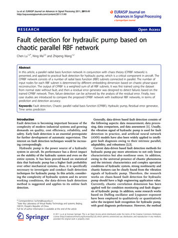
Lu et al. EURASIP Journal on Advances in Signal Processing 2011, /1/49based on neural network in conjunction with chaos theory has rarely appeared, especially for the fault detectionof hydraulic pump [4-7].Among several types of neural networks, radial basisfunction (RBF) network has relatively high convergencespeed, and can approximate to any nonlinear functions.It has been proved that RBF network has a very highperformance, in terms of nonlinear time series prediction, fault diagnosis in industrial systems, sensor andflight control systems, etc. [8-14].A CPRBF network for fault detection of hydraulicpump is presented in this article. This CPRBF networkwas first trained using the dataset from the normal statewithout fault of hydraulic pump, and then a residualerror generator was designed to detect several types offailures of hydraulic pump based on the trained CPRBFnetwork with one-step prediction of chaotic time series.The proposed model, based on Camastra and Colla’sapproach [15] and Yang et al.’ method [16], is able toreduce the effect of cumulative error and improve theprediction accuracy of RBF.This article is divided into three sections as follows:Section “Phase-space reconstruction of chaotic time series” describes the chaotic theory on phase space reconstruction employed to obtain the estimation ofcorrelation dimension. Section “Model of chaotic timeseries prediction and fault detection” proposes a newCPRBF network for chaotic time series prediction, and aresidual error generator based on CPRBF network wasalso designed to detect fault. Then, Section “Case studies” gives several case studies, including simulationresults of one-step iterative prediction and experimentalresults of fault detection for hydraulic pump.Phase-space reconstruction of chaotic time seriesAn important issue in the study of dynamic systems isthe dynamic phase-space reconstruction theory discovered by Packard et al. in 1980 [17]. It regards a onedimensional chaotic time series as the compressed information of high-dimensional space. The time series x(t), t 1,2,3,.,N can be represented as a series of points X(t)in a m-dimensional spaceX (t) (x (t) , x (t 1) , · · · , x (t (m 1)))(1)where m is called as the system embedding dimension.In particular, Takens’ embedding theory [18] states that,to obtain a dependable phase-space reconstruction ofdynamics system, it must bem 2D 1(2)where D is the dimension of system attractor. In orderto obtain a correct system embedding dimension,Page 2 of 10starting from the time series, it is necessary to estimatethe attractor dimension D.Among the different dimension definitions, correlationdimension discovered by Grassberger and Procaccia in1983 [19], is the most popular one due to its calculationsimplicity. It is defined as the following. If the correlation integral Cm(r) is defined as 2H r Xi Xj N (N 1)NCm (r) N(3)i 1 j i 1where H is the Heaviside function, m is the embedding dimension, and N is the number of vectors inreconstructed phase space. It is proved that if r is sufficiently small, and N would be sufficiently large, the correlation dimension D is equal toD limr 0ln (Cm (r))ln (r)(4)The algorithm plots a cluster of lnCm(r)-ln(r) curvesthrough increasing m until the slope of the curve’s linear part is almost constant. Then, the correlationdimension estimation D can be attained using leastsquare regression.Model of chaotic time series prediction and faultdetectionIn practice, it is difficult to get the exact estimationvalue of the minimum embedding dimension throughG-P algorithm. Furthermore, a single RBF network usesthe estimation value of minimum embedding dimensionas the number of its input, usually resulting in an inaccurate output due to the inaccurate estimation ofembedding dimension from human factor. Therefore, aPRBF network consisting of multiple RBF subnets isproposed to increase the system performance withdecreased error.Structure of CPRBFThe CPRBF is constituted of multiple RBF networksconnected in parallel for time series prediction. Thestructure of a CPRBF is shown in Figure 1.The CPRBF consists of n RBF subnets, which aredenoted as sub-RBF i (i 1,2,.,n), respectively. Eachsub-RBF subnet realizes one-step prediction independently at t 1. After the training of sub-RBF by historical dataset, one-step predicted value x̂i (t 1) can beobtained. The final predicted value x̂ (t 1) of PRBF canbe achieved through proper weighted combination ofx̂i (t 1).Input nodes of subnetEstimation value of the minimum embedding dimensionis regarded as the number of input nodes in the central
Lu et al. EURASIP Journal on Advances in Signal Processing 2011, /1/49sub RBF1sub RBF2Calculation of weighted factorsxˆ1 t 1xˆ2 t 1Z1Z2xˆ3 t 1sub RBF3Page 3 of 10Z3 xˆ t 1It is necessary to employ weighted factor ω to gain reasonable prediction result because each RBF subnet hasdifferent influence on the prediction process. In thisarticle, the optimal weighted value of each subnet isdetermined according to the minimum predicted absolute percent error (APE) of x̂i (t 1) in each case. Theoutput of PRBF net is the weighted sum of each individual RBF subnet, and the final predicted result can berepresented by the following equation.Znx̂ (t 1) n i x̂i (t 1)(7)i 1where x̂i (t 1) is the output of ith subnet, andx̂ (t 1) is the output of CPRBF network. Then, the leastsquare algorithm is employed to calculate the optimalweighted factors.sub RBFnxˆn t 1Figure 1 Structure of CPRBF.subnet, and each of other subnets uses different numbers (calculated based on m) as its input size.Once the correlation dimension D is obtained by G-Palgorithm and least square regression, the number ofinput nodes in the center subnet sub-RBF [n/2] can bedetermined asIn[n/2] [2D 1](5)where [·] denote an operator of rounded-up, and n isthe total number of subnets in PRBF. Ini is the numberof input nodes of subnet RBFi. When i [n/2], the subRBFi subnet is called the central subnet. Then, the number of input nodes of each subnet can be defined as Ini In[n/2] i n/2(6)In this article, each subnet RBFi uses the default parameters: the number of hidden layer is one, and thenumber of hidden nodes is equal to the number ofinput vectors.min JCPRBF minN [x̂(t 1) t 1n 2ωi x̂i (t 1)](8)i 1where N is the number of samples.Residual error generatorResidual error generator can be designed for fault detection optimization based on CPRBF network and CPRBFprediction process, and it provides a basis for the analysis and calculation of the model uncertainty robustness.The structure of a residual error generator is shown inFigure 2, where x(t) is the time series which can beobserved of actual system, CPRBF is the residual errorgenerator model trained using the dataset under normalstate, x̂(t) is the one-step prediction value of system,and e(t) is the output of residual error generator.Evaluation of residual errorResidual error evaluation is an important step of faultdetection. In this article, threshold selector is adopted toevaluate the residual error. The concept of thresholdselector is firstly introduced systematically in [20] tox 1 , x2 , , xmxˆ(t )x(t )Figure 2 Structure of residual error generator based on CPRBF network.e(t)
Lu et al. EURASIP Journal on Advances in Signal Processing 2011, /1/49solve the residual error evaluation problem of LTI systems with model uncertainty. The diagnostic decision isobtained based on the following rule:reval Jth fault state detectedreval Jth normal statewhere reval is a function related to residual error signaland employed to measure its deviation value, Jth is thethreshold.The variance of residual error signal can be adopted asresidual error evaluation function.1 (ei (t) E(e(t)))2n 1nreval i 1Figure 3 Process of fault detection.(9)Page 4 of 10The corresponding standard of threshold value canalso be determined based on diagnostic experiences inconjunction with different working conditions.Process of fault detectionProcess of fault diagnosis based on CPRBF and residualerror generator is shown in Figure 3.The detailed process is described as below: Step 1. Normalize the original time series fromdiagnosed system Step 2. Determine the number of input nodes ofeach subnet in CPRBF according to G-P algorithmand Takens’ theory
Lu et al. EURASIP Journal on Advances in Signal Processing 2011, /1/49Page 5 of 10 dx σ x σ ydy xz rz y dz xy bz Step 3. Determine weighted factor ω based on theone-step prediction result of each subnet Step 4. Calculate the final one-step prediction output of CPRBF Step 5. Construct a residual error generator, andcalculate the residual error according to the predicted output and the corresponding system output Step 6. Choose a residual error evaluation functionwith a threshold standard Step 7. Fault can be detected based on the evaluation function, with a fault alarm, once the residualerror exceeds the threshold value.(10)where s 16, r 45.95, b 4. 1,000 points of X-component Lorenz time series data were first normalizedand used for the following prediction.According to G-P algorithm, a cluster of lnCm(r)-ln(r)curves is plotted with the increase of the embeddingdimension m. The correlation dimension can be determined correspondingly, D 1.7643. According to Equation 2, m 5 (Figure 4).As a whole, 1,000 points were divided into two groups(training and testing dataset). The first 800 sampleswere used for RBF network training. The next 100 samples were used to determine the optimal weighted factorω, and the last 100 samples for testing of the predictionaccuracy between RBF and CPRBF. The number ofinput nodes of central subnet in the PRBF was 5,obtained from the estimation of the minimum embedding dimension. After the training of each subnet, theoptimal weighted factor ω can be obtained via leastsquare algorithm. The parameters of CPRBF are listedas below.Case studiesVerification results of one-step iterative predictionConsidering the lack of practicability from a commonone-step prediction method, one-step iterative prediction should be adopted to verify the prediction performance instead. In general, each predicted result at Step4 is consecutively used as the next input data to achieveone-step iterative prediction. The future trend of actualcase (Lorenz’s attractor, hydraulic pump) can beobtained gradually with the repetition of Steps 3 and 4,and the loop times depends on the length of actualexpected data.In[n/2] 5;Simulation of Lorenz’s attractorInin [3, 4, 5, 6, 7]; [0.0181 0.0196 0.8829 0.0749 0.000]Figure 5 shows the one-step iterative predicted resulton the last 100 points of Lorenz’s time series by CPRBFnetwork. Figure 6 shows the comparison on APE of Lorenz time series between RBF and CPRBF.In this section, the simulation result of Lorenz’s attractor data is given to verify the performance of the proposed method. Equation 10 is employed to generate theLorenz’s time series data.0-0.5-1-1.5ln C m (r)m 2-2-2.5m 9-3-3.5-4-4.5-2.5-2-1.5-1-0.5lnrFigure 4 Plot of lnCm(r)-ln(r) of Lorenz time series.00.51
Lu et al. EURASIP Journal on Advances in Signal Processing 2011, /1/49Page 6 of 1030Pre-dataOrg-data20 X 100-10-20-300102030405060Lorenz’s time series708090100Figure 5 One-step iterative predicted result of Lorenz time series.Figures 5 and 6 prove that: One-step iterative prediction based on CPRBF network has good prediction performance Comparing with RBF network, CPRBF network hasbetter performance on iterative prediction, in termsof convergence and stability.Experimental result using real data of hydraulic pumpIn this section, several groups of time series data (normaland fault conditions) were generated from a test rig ofSCY Hydraulic pump. Table 1 shows the correspondingmaximum Lyapunov exponents (lmax) of the above timeseries. Because all lmax values are positive, the experimental data can be regarded as chaotic time series.According to G-P method, a cluster of lnCm(r)-ln(r)curves for Data 1 is plotted with the increase of theembedding dimension m as shown in Figure 7. The correlation dimension can be determined correspondingly,D 2.2346. According to Equation 2, m 6 (Figure 7).In this case, 800 points of time series data from thevibration signal of hydraulic pump were used for prediction. As a whole, 800 data points were divided intotraining and testing dataset. The first 600 samples wereemployed for RBF network training, the next 100 samples for the determination of the optimal weighted factor ω, and the last 100 samples for testing of predictionaccuracy between RBF and PRBF. The number of inputnodes (minimum embedding dimension) is 5 accordingto the aforementioned approach. After the training ofeach subnet, the weighted factor ω can also be obtained.The parameters of CPRBF areIn[n/2] 6;Inin [4, 5, 6, 7, 8]; [0.0000 0.1610 0.2221 0.2886 0.3283]Figure 8 shows the result using one-step iterative prediction based CPRBF network. Figure 9 presents thecomparison of APE error between RBF and CPRBF, andboth are all based on Data 1.Comparing with RBF network, PRBF model has higherprediction accuracy, without the effect of erroraccumulation.Experimental results of fault detection for hydraulicpumpConstruction of detection model using CPRBFAccording to the G-P method, a cluster of lnCm(r)-ln(r)curves of normal data is plotted with the increase of the1.2PRBFRBFAPE Value10.80.60.40.200102030Figure 6 Comparison of APE between RBF and CPRBF.405060Absolute Error Series708090100
Lu et al. EURASIP Journal on Advances in Signal Processing 2011, /1/49Table 1 Lyapunovs of hydraulic pump’s sample ding dimension m, as shown in Figure 10. Thecorrelation dimension can be determined correspondingly, D 2.2472. According to Equation 2, m 6.In this case, 800 points of time series data from thevibration signal without fault were used for the construction of detection model. As a whole, 800 datapoints were divided into training and testing dataset.The first 600 samples were employed for network training, the next 100 samples for the determination of theoptimal weighted factor ω, and the last 100 samples fordetermination of the threshold of fault detection. Aftertraining and testing, prediction model of normal statecan be determined. The parameters of CPRBF areshown as below.In[n/2] 6; [0.0462 0.0000 0.3696 0.3558 0.2283]Inin [4, 5, 6, 7, 8];Figure 11 shows the residual error of normal data, andCPRBF based model has better prediction performancewith an accuracy of about 10-6.Residual error signals of hydraulic pump based on CPRBFnetworkWear fault of valve plate Dry friction is probablycaused by fatigue crack, surface wear, or cavitation erosion, etc. In case of this failure, with the increasing ofmoment coefficient between rotor and valve plate, contact stress grows and oil film becomes thinner. Further,as a repetitive impact of the contact stress, the surfaceof valve plate is fatigued and spalls. As a result, dry friction appears, with an increment of motion gap ofhydraulic pump and a decrement of volumetric efficiency. Meanwhile, the dry friction inevitably generates0-1lnCm(r)-2m 2-3-4m 15-5-6-7-2.5-2-1.5-1-0.500.51lnrFigure 7 Plot of lnCm(r)-ln(r) of hydraulic pump’s sample data.Page 7 of 10additional vibration signals in the valve plate’s shell nearthe high pressure chamber.In this article, 100 points of time series data from thevibration signal with valve plate rotor wear were usedfor detection according to the aforementioned method.Figure 12 shows the residual error of valve plate rotorwear.Wear fault between swash plate and slipper Dry friction, caused by oil impurities or small holes on plungerball, etc., usually results in wear or burnout of the fayingsurface between swash plate and slipper, which probablycauses the falling of slipper, and affects the performanceof hydraulic pump.Similar to the above case study, 100 points of timeseries data from the vibration signal with wear faultbetween swash plate and slipper of hydraulic pumpwere used for fault detection. Figure 13 shows the residual error of wear fault between swash plate and slipper.Fault detectionThreshold value is a key point in fault decision-making,due to uncertainties in practical and external disturbances. The rate of fail-to-report increases if the threshold is too large, vice versa, the rate of false alarm wouldincrease. Appropriate threshold should be selectedaccording to the analysis, with the support of residualerror evaluation function proposed, on hydraulic pump’snormal and faulty data.Two groups of normal data and six groups of faultydata from a testing hydraulic pump were used for analysis. Residual error series were obtained, respectively,via residual error generator designed using CPRBF network, and each variance of residual error series wascalculated correspondingly. Table 2 shows the variancevalues.It can be seen obviously from Table 2 that, two magnitude levels of residual error’s variance values betweennormal and fault states are clearly distinct. According toexperience, the threshold can be determined with astandard of 10 times higher than the mean of variancesunder normal states. Here, Jth 3.196e-005. It should bealso noticed that, the threshold standard must be readjusted according to different working conditions.The variance values of the above two cases are3.7781e-004 and 1.7305e-004, respectively. These valuesare greater than J th , thus, the fault can be detectedbased on the variance of residual error signal.ConclusionsIt is shown from the simulation results that, CPRBF network model, in conjunction with phase space reconstruction, show better capabilities and reliability inpredicting chaotic time series, as well as a high performance of convergence ability and prediction precisionon short-term prediction of chaotic time series.
Lu et al. EURASIP Journal on Advances in Signal Processing 2011, /1/49Page 8 of 10one-step iterative prediction of the fault time series0.03Pre-dataOrg-dataAcceleration (m/s2)0.020.010-0.01-0.02-0.030102030405060Chaotic Time Series708090100Figure 8 One-step iterative predicted result of Data1.0.01PRBFRBFAPE Value0.0080.0060.0040.00200204060Abslute Error Series80100Figure 9 Comparison of APE between RBF and CPRBF.The experimental results show that, CPRBF model hashigh ability in approximation to the output and state ofa normal system, which is useful for fault detection. TheCPRBF network can memorize various nonlinear statesor interferences of a system with normal states,therefore, the actual system output will be different withthe predicted output of CPRBF network once any anomaly occurs, and the system can be regarded as faultystate if the residual error exceeds the threshold. Thus,CPRBF network based method is effective to real-time0lnCm(r)-2m 2-4-6m 10-8-10-12-3-2.5-2-1.5-1lnrFigure 10 Plot of lnCm(r)-ln(r) of hydraulic pump’s data.-0.500.51
Lu et al. EURASIP Journal on Advances in Signal Processing 2011, /1/49Page 9 of 100.060.04Amplitude(m/s 2)0.020-0.02-0.04-0.0601020304050Time Series6070809010020304050Time Series60708090100Figure 11 Residual error of normal data.0.060.04Amplitude(m/s 2)0.020-0.02-0.04-0.06010Figure 12 Residual error of valve plate rotor wear.0.030.02A m p litu d e (m / s 2 )0.010-0.01-0.02-0.0301020304050Time SeriesFigure 13 Residual error of wear fault between swash plate and slipper.60708090100
Lu et al. EURASIP Journal on Advances in Signal Processing 2011, /1/49Page 10 of 10Table 2 Variance values of residual error seriesStateResidual error signalDataNormal 1Normal 2Fault 1Fault 2Fault 3Fault 4Fault 5Fault 62.5383Mean of variance3.91625Normal (e-006)Fault (e-004)1.651467fault detection. However, it is also shown from theexperiments that different types of faults might represent the same fault form, accordingly, the proposedmethod is not suitable for performing fault location butfor conducting condition monitoring. Further work willfocus on how to isolate any type of fault and identify itsfault classification.This article mainly aims to discuss the feasibility andpossibility of practical fault detection for hydraulicpump using neural network in conjunction with chaostheory. A commonly used neural network in the pastand now, namely, RBF network was employed for faultdetection for hydraulic pump in conjunction with chaostheory. Certainly, methods using chaos theory combinedwith other popular ANNs should be also our emphasisin the following works. As known, support vectormachine (SVM) has been widely applied in many fields.Compared with other ANNs, SVM overcomes manydefects, such as over-fitting, local convergence. In addition, SVM has advantages over other ANNs, in terms ofrobustness and prevention of curse of dimensionality,etc. Thus, our further work will focus on SVM in conjunction with chaos theory, especially for those edgementsThe research is supported by the National Natural Science Foundation ofChina (Grant Nos. 61074083, 50705005), as well as the TechnologyFoundation Program of National Defense (Grant No. Z132010B004). Theauthors are also very grateful to the reviewers and the editor for theirvaluable suggestions.Author details1State Key Laboratory of Virtual Reality Technology and systems, Beijing,100191, People’s Republic of China 2School of Reliability and SystemsEngineering, Beihang University, Beijing, 100191, People’s Republic of China3Department of Foundation Science, The First Aeronautical Institute of AirForce, Xinyang 464000, People’s Republic of China15.16.17.18.19.Competing interestsThe authors declare that they have no competing interests.Received: 27 December 2010 Accepted: 30 August 2011Published: 30 August 2011References1. KY Chen, CP Lim, WK Lai, Application of a neural fuzzy system with ruleextraction to fault detection and diagnosis. J Intell Manuf. 16, 679–691(2005). doi:10.1007/s10845-005-4371-120.MM Hanna, A Buck, R Smith, Fuzzy petri nets with neural networks tomodel products quality from a CNC-milling machining centre. IEEE TransSyst Man Cyber A 26, 638–645 (1996). doi:10.1109/3468.531910MM Polycarpou, AJ Helmicki, Automated fault detection andaccommodation: a learning system approach. IEEE Trans Syst Man Cyber.25, 1447–1458 (1995). doi:10.1109/21.467710WL Jiang, DN Chen, CY Yao, Correlation dimension analytical method andits application in fault diagnosis of hydraulic pump. Chin J Sens Actuators17(1), 62–65 (2004)WL Jiang, YM Zhang, HJ Wang, Hydraulic pump fault diagnosis methodbased on lyapunov exponent analysis. Mach Tool Hydraulics 36(3), 183–184(2008)QJ Wang, XB Zhang, HP Zhang, Y Sun, Application of fractal theory of faultdiagnosis for hydraulic pump. J Dalian Maritime Univ. 30(2), 40–43 (2004)YL Cai, HM Liu, C Lu, JH Luan, WK Hou, Incipient fault detection for plungerball of hydraulic pump based on Duffing oscillator. Aerosp Mater Technol.39(suppl), 302–305 (2009)J Park, IW Sandberg, Universal approximation using radial-basis-functionnetworks. Neural Comput. 3(2), 246–257 (1991). doi:10.1162/neco.1991.3.2.246T Poggio, F Girosi, Networks for approximation and learning. Proc IEEE.78(9), 1481–1497 (1990). doi:10.1109/5.58326S Chen, Nonlinear time series modeling and prediction using Gaussian RBFnetworks with enhanced clustering and RLS learning. Electron Lett. 31(2),117–118 (1995). doi:10.1049/el:19950085MAS Potts, DS Broomhead, Time series prediction with a radial basisfunction neural network. SPIE Adapt Signal Process. 1565, 255–266 (1991)KG Narendra, VK Sood, K Khorasani, R Patel, Application of a radial basisfunction (RBF) neural network for fault diagnosis in a HVDC system. IEEETrans Power Syst. 13(1), 177–183 (1998). doi:10.1109/59.651633DL Yu, JB Gomm, D Williams, Sensor fault diagnosis in a chemical processvia RBF neural networks. Control Eng Practice 7(1), 49–55 (1999).doi:10.1016/S0967-0661(98)00167-1YM Chen, ML Lee, Neural networks-based scheme for system failuredetection and diagnosis. Math Comput Simul. 58(2), 101–109 (2002).doi:10.1016/S0378-4754(01)00330-5F Camastra, AM Colla, Neural short-term prediction based on dynamicsreconstruction. Neural Process Lett. 9, 45–52 (1999). doi:10.1023/A:1018619928149HY Yang, H Ye, GZ Wang, MY Zhong, A PMLP based method for chaotictime series prediction, in Proceedings of the 16th IFAC World Congress, MoE11-To/2 (2005)N Packard, J Crutcheld, J Farmer, R Shaw, Geometry from a time series.Phys Rev Lett. 45, 712–716 (1980). doi:10.1103/PhysRevLett.45.712F Takens, Detecting strange attractors in turbulence. Dynamical Systemsand Turbulence, Warwick 1980, Lecture Notes in Mathematics 898 (Springer,Berlin) 366–381 (1981)P Grassberger, I Procaccia, Measuring the strangeness of strange attractors.Physica D9, 189–208 (1983)A Emami-Naeini, MM Akhter, SM Rock, Effect of model uncertainty onfailure detection: the threshold selector. IEEE Trans Autom Control 33,1106–1115 (1988). te this article as: Lu et al.: Fault detection for hydraulic pump basedon chaotic parallel RBF network. EURASIP Journal on Advances in SignalProcessing 2011 2011:49.
Hydraulic pump is the power source of a hydraulic system in aircraft. Its performance has a direct impact on the stability of the hydraulic system and even on the entire system. It has been proved based on statistical data that hydraulic pump has a higher fault probability over other mechanical systems, thus, it is specifically