Transcription
Finance and Economics Discussion SeriesDivisions of Research & Statistics and Monetary AffairsFederal Reserve Board, Washington, D.C.Measuring Counterparty Credit Exposure to aMargined CounterpartyMichael S. Gibson2005-50NOTE: Staff working papers in the Finance and Economics Discussion Series (FEDS)are preliminary materials circulated to stimulate discussion and critical comment. Theanalysis and conclusions set forth are those of the authors and do not indicateconcurrence by other members of the research staff or the Board of Governors.References in publications to the Finance and Economics Discussion Series (other thanacknowledgement) should be cleared with the author(s) to protect the tentative characterof these papers.
Measuring Counterparty Credit Exposure to a Margined CounterpartyMichael S. Gibson September 2005Risk Analysis Section, Division of Research and Statistics, Federal Reserve Board. This paper representsthe views of the author and should not be interpreted as reflecting the views of the Board of Governors of theFederal Reserve System or other members of its staff. I can be reached via email at michael.s.gibson@frb.gov.Postal address: Mail Stop 91, 20th and C Streets NW, Washington, DC 20551. Phone: 1-202-452-2495.
Measuring Counterparty Credit Exposure to a Margined CounterpartyAbstract: Firms active in OTC derivative markets increasingly use margin agreements toreduce counterparty credit risk. Making several simplifying assumptions, I use both a quasianalytic approach and a simulation approach to quantify how margining reduces counterpartycredit exposure. Margining reduces counterparty credit exposure by over 80 percent, usingbaseline parameter assumptions. I show how expected positive exposure (EPE) depends onkey terms of the margin agreement and the current mark-to-market value of the portfolio ofcontracts with the counterparty. I also discuss a possible shortcut that could be used by firmsthat can model EPE without margin but cannot achieve the higher level of sophisticationneeded to model EPE with margin.Keywords: counterparty risk, collateral, margin, derivatives
1IntroductionFirms active in OTC derivative markets increasingly use margin agreements to reduce counterparty credit risk. Making several simplifying assumptions, I use both a quasi-analyticapproach and a simulation approach to quantify how margining reduces counterparty creditexposure. I show how expected positive exposure (EPE) depends on key terms of the margin agreement and the current mark-to-market value of the portfolio of contracts with thecounterparty. I also discuss a possible shortcut that could be used by firms that can modelEPE without margin but cannot achieve the higher level of sophistication needed to modelEPE with margin.1.1 Counterparty credit riskA firm that uses OTC derivatives is exposed to counterparty credit risk because a counterparty may default when the portfolio of OTC derivative contracts with the counterpartyhas positive value. The value of an OTC derivatives portfolio, which depends on marketvariables such as interest rates or exchange rates, will change when those variables change.As a result, counterparty credit exposure will change in the future even if no new positionsare added to the portfolio.Because future counterparty credit exposure is uncertain, measuring it requires a statisticalforecast of future moves in market variables. With such a forecast in hand, a dealer canestimate the probability distribution of counterparty credit exposure on one or more futuredates. Summary measures of counterparty credit exposure can be computed from theseprobability distributions.Three commonly used summary measures, as defined by BCBS (2005), are Potential future exposure (PFE): the maximum exposure estimated to occur on afuture date at a high level of statistical confidence.Expected exposure (EE): the probability-weighted average exposure estimated to existon a future date.Expected positive exposure (EPE): the time-weighted average of individual expectedexposures estimated for given forecasting horizons (e.g. one year). Both industry experts and regulators agree that EPE is the conceptually correct measureof exposure to be used in a calculation of economic or regulatory capital for counterpartycredit risk.1 For that reason, I focus on measuring the effect of margining on EPE. However,the techniques presented here could be adapted to measure PFE.1.2 Margin agreementsMore and more participants in OTC derivatives markets use collateral and margin agreementsto reduce counterparty credit risk. According to a recent survey, 55 percent of derivatives1Canabarro and Duffie (2003), Picoult and Lamb (2004), BCBS (2005).1
transactions are covered by margin agreements as of December 31, 2004, up from 30 percentas of December 31, 2002.2A margin agreement contains rules for computing the amount of collateral to be passedbetween parties on any given day. There are several key terms that are individually negotiatedby counterparties. The models I present below consider four key terms:Threshold: Exposure amount below which no margin is held.Grace period: Number of days after default until the counterparty’s position is liquidatedor replaced.Remargin period: Interval (in days) at which margin is monitored and called for.Minimum transfer amount: Amount below which no margin transfer is made.The grace period used in a model should be based on market practice and experience inclosing out defaulted counterparties, not solely on the grace period written into the marginagreement.While margin agreements can reduce counterparty credit risk, they pose a challenge tomodelers. Models to measure counterparty credit risk are already notoriously complicatedand difficult, because they must forecast future moves in market variables into the distantfuture (as long as 30 years, for long-dated swap contracts) and they must be able to revaluethe portfolio of derivative contracts given arbitrary changes in market variables. Marginagreements add another layer of complexity, because future collateral amounts and margincalls must also be modeled.3While a great deal of work has been done in recent years to improve understanding of EPE forunmargined counterparties, little has been done for margined counterparties.4 By building asimplified, stylized model of EPE for a margined counterparty, I aim to fill this gap in theliterature by establishing how EPE varies with a few key terms of a margin agreement aswell as with the current mark-to-market value of the contracts with the counterparty. I alsodiscuss what shortcuts may be appropriate for firms that can model EPE without marginbut cannot achieve the higher level of sophistication needed to model EPE with margin.2Measuring EPE for a margined counterpartyThe most common models for measuring EPE are simulation models. These models have foursteps. First, simulate a sample path for the future values of the market variables underlyingthe portfolio of derivative contracts with a counterparty.5 Second, compute the mark-tomarket value of the portfolio along the path. Third, compute exposure as the mark-to-market2ISDA (2005)Margin agreements also give rise to operational and legal risks that must be managed.4Work on EPE for unmargined counterparties includes ISDA (2001, pp. 63–69), Canabarro, Picoult andWilde (2003), Canabarro and Duffie (2004).5The correct portfolio to use when computing counterparty exposure is a “netting set.” As defined inBCBS (2005), “a ‘netting set’ is a group of transactions with a single counterparty that are subject to alegally enforceable bilateral netting arrangement . . . If a transaction with a counterparty is not subject to abilateral netting agreement, it comprises its own netting set.”32
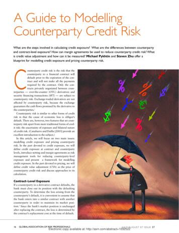
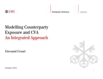
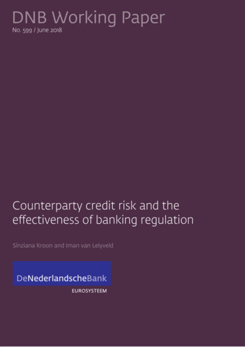
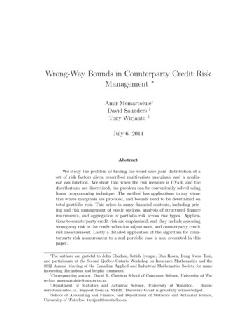
value, if positive, or zero otherwise. Fourth, average exposure across sample paths and overtime to compute EPE.6A margin agreement requires additional modeling.7 At each time step along the sample path,the model must test whether a margin call is required or whether excess collateral shouldbe returned to the counterparty. If a margin call is made, the model must track the deliveryof the collateral. When considering counterparty default, the model must consider whethermargin calls made on the previous day have been received yet. All these add complexity tothe EPE model.I build a simplified, stylized model of EPE for a margined counterparty. I consider both aquasi-analytic model and a slightly richer simulation model. The model assumes that themark-to-market value of the portfolio of contracts with the counterparty follows a randomwalk with Gaussian increments. The model considers only four key terms of a margin agreement. The mechanics of margin calls are simplified for tractability. The model does notallow for initial margin or non-cash collateral.8 Sections 3 and 4 describe the analytic andsimulation models in more detail.The “base case” values that I assume for the four key terms of a margin agreement, as wellas for the current mark-to-market (MTM) value of the contracts with the counterparty, areshown in the table below. In addition, I set the annualized standard deviation of the futureMTM value of the contracts with the counterparty equal to one. Because EPE scales withthe standard deviation, this is simply a normalization.ParameterBase case valueCurrent MTM0Threshold0Grace period10 daysRemargin period1 dayMinimum transfer amount*0* used in simulations, not used in analytic approximation2.1 ResultsOne summary measure of the effect of margining is the ratio of EPE taking margining intoaccount to EPE without margining. For the base case parameters given in the table above,this ratio equals 0.17 in both the analytic approximation and the simulations. Put anotherway, a margin agreement with standard terms can reduce counterparty credit exposure byover 80 percent.Figures 1 and 2 show how EPE depends on the key terms of the margin agreement andthe current MTM. Each panel varies one parameter while holding the other four at their6The basic structure of an EPE model is described in Canabarro and Duffie (2004).I consider one-sided margin agreements, where only one party to the margin agreement (the counterparty) is ever required to provide collateral.8Allowing non-cash collateral would make the model more realistic. However, according to ISDA (2005),cash makes up 73 percent of collateral held against OTC derivative exposures.73
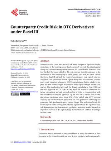
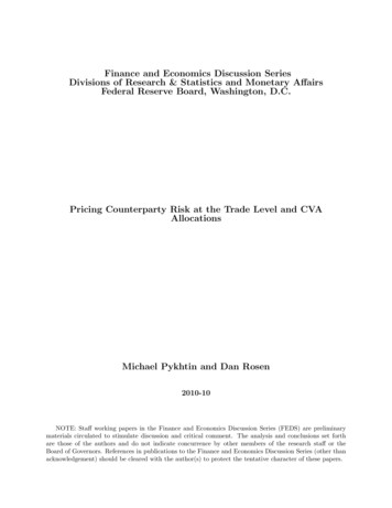
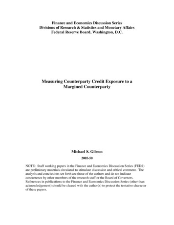
base case values. Figure 1 plots the ratio of EPE with margin to EPE without marginwhile Figure 2 plots the levels of EPE with and without margin (blue solid and red dashedlines, respectively).9 The figures show both the analytic approximation (left column) andsimulations (right column).The top panels of Figures 1 and 2 show how EPE varies with the current MTM of theportfolio. Comparing EPE without and with margining (the red and blue lines in the toppanel) in Figure 2, margining removes nearly all of the strong dependence of EPE on currentMTM that exists without margining. Figure 1 shows that portfolios with large current MTMshow the greatest reduction in EPE from margining.The second row of panels in Figures 1 and 2 shows how EPE varies with the collateralthreshold. EPE with margining increases strongly with the threshold, with the effect onlytapering off when the threshold is so high that EPE with margining nears EPE withoutmargining.The two top rows of figures 1 and 2 show how EPE varies individually with the currentMTM and the collateral threshold. There are interesting interactions when these are variedsimultaneously, as shown in Figure 3. In this figure, all other parameters are at their basecase values. At high levels of current MTM, the threshold has a linear effect on EPE. Atlow levels of current MTM, the threshold has almost no effect on EPE. At low thresholds,current MTM has almost no effect on EPE. At high thresholds, EPE increases linearly withcurrent MTM up to the threshold, then flattens out.The third and fourth rows of Figures 1 and 2 show how the grace period and the remarginperiod affect EPE. In general, EPE increases as both the grace period and remargin periodget longer. However, the effect is not identical, and the difference can be understood as dueto the timing of a default within the period. A default always occurs at the beginning of thegrace period, and exposure can rise during the entire grace period until, at the end of thegrace period, the position is closed. In contrast, a default will occur at a random time duringthe remargin period. On average, exposure will have risen without remargining for half ofthe remargin period before a default.For both the grace period and the remargin period, Figure 1 shows the square root of timefunction, plotted as a red dashed line. The square root of time is added to the plot to reflectthe idea that EPE with margin could be approximated by multiplying 1-year EPE withoutmargin by the square root of the grace period. This approximation appears to work well.For the reasons discussed above, EPE rises more slowly than the square root of time for theremargin period.Figure 4 varies the grace period and remargin period simultaneously. The lack of muchcurvature in the EPE surface in Figure 4 suggests that there is little interaction between thetwo in their effect on EPE.The results in Figures 1, 2, and 4 set both the current MTM and threshold to zero. Moregenerally, when the current MTM or threshold is not zero, EPE will reflect both current and9EPE without margin (the denominator of the ratios shown in Figure 1) is EPE computed at the basecase values without margining, except that the EPE without margin is recomputed for each value of currentMTM.4
future exposure. Only the future exposure piece, but not the total EPE, would be expectedto increase with the grace period or remargin period.The bottom panel in Figures 1 and 2 shows how EPE varies with the minimum transferamount. Only the simulations allow for a non-zero minimum transfer amount. As expected,EPE rises with the minimum transfer amount, but quite slowly.2.2 Summary, and a possible shortcut EPESome firms may be able to model EPE without margining but may not have the higherlevel of sophistication to model EPE with margining. In looking for a possible shortcut EPEfor such firms, the figures lead to the following conclusions about the effects of each of thevariables: The collateral threshold and the current mark-to-market have important effects onEPE for margined counterparties. These effects should be taken into account in anyshortcut EPE calculation.The grace period has an effect on EPE that is roughly proportional to the square rootof time (when the current mark-to-market and threshold are zero, as they are in theBase Case).The remargin period has an effect similar to the grace period, but slightly weaker.If the minimum transfer amount is small, it has little effect on EPE and, if a smallamount of conservatism were added on to the shortcut EPE to cover it, it may not bematerial. Analyzing Figure 3 suggests using the threshold plus the 10-day expected exposure (EE)computed with no margining as a shortcut EPE with margining.10 Note that the shortcutuses expected exposure after 10 days (EE), not 10-day expected positive exposure (EPE),which is the average exposure over the first 10 days. For a margined counterparty, exposureis only relevant at the end of the 10 day grace period, so expected exposure—which measuresexposure on a single future date—is the relevant concept, not EPE—which averages exposureover many future dates. As part of the shortcut calculation, if the EPE computed withoutany threshold (implying no margining would ever take place) were smaller than the proposedshortcut EPE, it could be used instead. It would not make sense to have a higher loanequivalent amount for a margined counterparty than for an otherwise-identical unmarginedcounterparty.The suggested shortcut EPE formula is shown in Table 1. Panel A shows the shortcutformula, while Panel B shows the analytic EPE numbers from Figure 3. As hoped for, theshortcut EPE shown in Panel A is conservative – it is always greater than the actual EPE inPanel B – but it is fairly sensitive to the two key risk drivers (current mark-to-market andthreshold).10If the grace period were more than 10 days, “10-day EE” would be replaced with the EE for thelonger grace period. If remargining were less frequent than daily, the 10-day period should be lengthenedaccordingly.5
3The analytic approximationBy making some simplifying assumptions, it is possible to obtain a quasi-analytic approximation for EPE to a margined counterparty as a function of the parameters given in thetable above.113.1 Definitions and notation time t runs from today, t 0, to the EPE horizon, t TV (t) mark-to-market at time tC(t) collateral held at tE(t) exposure at t max(0, V (t) C(t))D collateral thresholdm grace periodrm remargin periodEE(t) expected exposure at t conditional on default at t average of E(t default)over possible values of V (t) EP E average of EE(t) over (0, T )For a non-defaulting counterparty, collateral held is defined byC(t) max(0, V (s) D)(1)where s is the remargin date at or before t. Assuming that today (t 0) is a remargin date,s t t mod rm. For the base case of daily remargining, rm 1 and s t. I also assumefor the analytic approximation that collateral is monitored, called for, and delivered on eachremargin date.12Exposure at default is defined byE(t default) max(0, V (t m) C(t))(2)I assume that the stochastic behavior of V (t) is unaffected by the counterparty’s default, ineffect assuming no wrong-way risk.3.2 Deriving expected exposureSubstituting (1) into (2) givesE(t default) max(0, V (t m) max(0, V (s) D))Using (3), the expected exposure at t can be written asZEE(t) max(0, V (t m) max(0, V (s) D)) dF1112(3)(4)I use the term “quasi-analytic” because solving the model requires numerical integration.The simulation approach below assumes that collateral called on t is delivered on t 1.6
where F F (V (t m), V (s)) is the joint distribution of V (t m) and V (s).Looking at (3), the various max operators lead to four possible values of the exposure atdefault, depending on V (t m) and V (s), summarized in the following table:E(t default)V (s) DV (s) DV (s) DV (s) DV (t m) 0V (t m) 0V (t m) V (s) DV (t m) V (s) D0V (t m)0V (t m) V (s) DUsing this table, (4) can be rewritten asZEE(t) V (t m) dF V (s) D,V (t m) 0Z(V (t m) V (s) D) dF(5)V (s) D,V (t m) V (s) DTo establish the joint distribution F (V (t m), V (s)), I assume that V (t) follows a randomwalk with Gaussian increments: V (s) V (0) σ sX(6) (7)V (t m) V (0) σ sX σ t m sYwhere X and Y are independent standard normal random variables.Using this assumption and setting V (0) V for ease of notation, (5) can be rewritten asEE(t) Z ZD V σ s D V σ sZZ V σ sx σ t m s Dσ t m s (V σ sx σ t m sy) φ(x)φ(y) dy dx (8)(σ t m sy D) φ(x)φ(y) dy dxwhere φ() is the standard normal density function.Simplifying (8) a little bit to elimnate the double integrals yields ” “ sx 2 V σ sxσ t m s 21 σV σt m s EE(t) φ(x) dx(V σ sx)N eσ t m s2π “”2 DV Dσ t m s 21 σ t m sD N eDNσ sσ t m s2π(9)ZD V σ swhere N () is the standard normal cumulative distribution function.7
Equation (9) is the expression used to compute EE(t).13 Using (9), EP E is computed asZ1 TEE(t) dt(11)EP E T 0I used numerical integration to produce the analytic results shown in Figures 1–4, settingthe volatility parameter σ 1.4The simulation modelThe simulation model also assumes that the mark-to-market value of contracts in the nettingset follows a random walk with Gaussian increments.14 As changes in the mark-to-marketvalue cause changes in exposure, margin is called for when the mark-to-market exceeds thethreshold (or returned if the mark-to-market falls below the threshold).The simulation algorithm uses the following notation: V0 is the current mark-to-market. Eis the exposure gross of collateral, D is the threshold. C0 , the initial collateral held, equalsmax(0, V0 D). The grace period (days to liquidate a defaulted counterparty’s positions) ism. Collateral called on day t is assumed to be delivered on day t 1. Cit default is collateralavailable conditional on the counterparty’s defaulting at t. Eit default is mean exposure,net of collateral, conditional on default at t and taking into account the movement in themark-to-market over the grace period. ǫ is a standard normal random variable. The endpointof the simulation, T , equals 250 days (one year). The number of simulations, N , and thenumber of simulations of exposure within the grace period, M , are both set to 400.The simulation algorithm is:1: for i 1 to N do2:Vi0 V0 , Ci0 C03:for t 1 to T doq14:Vit Vit 1 ǫ 2505:Eit max(0, Vit )6:Cit Cit 1 Callit 17:if t is a remargining day then8:Callit max(Eit D, 0) Cit9:if Callit minimum transfer amount then10:Callit 013If s 0, equation (9) simplifies to “”2 V1 σ t m 2 σ t m V N V eσ t m2π“”2EE(t) 12 σ D t mσt m DN D e σ t m2πif V D(10)if V D14Since real-world contracts need not follow a random walk, a useful extension would be to repeat thesimulation exercise with a more realistic model for the mark-to-market value.8
11:end if12:end if13:Cit default CitP pmM14:Eit default M1 C defaultmax0,V ǫititj 125015:end for P16:EP Ei T1 Tt 1 max(0, Eit default)17: end forPN118: EP E Ni 1 EP EiThe definition of Cit default in line 13 assumes that collateral that was posted on t 1 isdelivered on t despite the counterparty’s default on t. An alternative would be to assumethat this collateral would be clawed back by the bankruptcy court before it is delivered on t.The alternative would change this line to Cit default min(Cit , Cit 1 ). The alternative hasa small effect on the results shown in Figures 1 and 2. In the base case, it increases the EPEwith margin by about 0.007, or 3 percent of EPE without margin.9
ReferencesBasel Committee on Banking Supervision, 2005. The Application of Basel II to Trading Activities and the Treatment of Double Default Effects. Basel: Bank for International Settlements (July). http://www.bis.org/publ/bcbs116.pdf [cited as BCBS (2005)].Canabarro, Eduardo and Darrell Duffie, 2003. Measuring and marking counterparty risk. InAsset/Liability Management of Financial Institutions, ed. Leo M. Tilman, InstitutionalInvestor Books.Canabarro, Eduardo, Evan Picoult, and Tom Wilde, 2003. Analysing counterparty risk.Risk 16:9 (September), 117–122.International Swaps and Derivatives Association, 2001. ISDA’s Response To The BaselCommittee On Banking Supervision’s Consultation On The New Capital Accord. http://www.isda.org/c and a/docs/BASELRESPONSEII08Board.pdf [cited as ISDA(2001)]International Swaps and Derivatives Association, 2005. ISDA Margin Survey 2005. http://www.isda.org/c and a/pdf/ISDA-Margin-Survey-2005.pdf [cited as ISDA (2005)]Picoult, Evan and David Lamb, 2004. Economic capital for counterparty credit risk. InEconomic Capital: A Practitioner Guide, ed. Ashish Dev, Risk Books.10
Figure 1. (EPE with margin)/(EPE without margin) as a function of current mark-to-market(MTM), threshold, grace period, remargin period and minimum transfer amount(the red dashed line plots the square root of time function)AnalyticSimulation0.40.40.20.20 101Current MTM230 1110.50.500123Threshold/EPE without margin400.60.60.40.40.20.20050100Grace period (days)00.60.60.40.40.20.20050100Remargin Period (days)0001Current MTM2123Threshold/EPE without margin050100Grace Period (days)050100Remargin Period (days)340.60.40.200123Minimum Transfer Amount/EPE without margin11
Figure 2. EPE for a margined counterparty as a function of current mark-to-market (MTM),threshold, grace period, remargin period and minimum transfer amount (reddashed line shows EPE without margin)AnalyticSimulation3322110 101Current MTM230 10.30.30.20.20.10.100123Threshold/EPE without margin400.30.30.20.20.10.10050100Grace period (days)00.30.30.20.20.10.10050100Remargin Period (days)0001Current MTM2123Threshold/EPE without margin050100Grace Period (days)050100Remargin Period (days)340.30.20.100123Minimum Transfer Amount/EPE without margin12
Figure 3. Analytic approximation to EPE with margin as a function of both threshold andcurrent mark-to-market13
Figure 4. EPE with margin as a function of grace period and remargin period14
Table 1. Shortcut EPE as a function of current mark-to-market and thresholdCurrent 00.0801.0802.0803.080Panel A: Shortcut 802.970Panel B: EPE measured with analytic approximation00.008 0.046 0.074 0.079 0.079 0.0790.07910.032 0.249 0.758 0.962 0.988 0.9900.99020.034 0.277 0.993 1.716 1.950 1.9781.98030.034 0.279 1.022 1.952 2.704 2.9402.968Memo:No threshold 0.034 0.279 1.024 1.982 2.970 3.9604.950Note: Shortcut EPE equals threshold plus 10-day expectedexposure (EE) or EPE for an unmargined counterparty (no threshold),whichever is smaller. Panel B uses daily remargining anda 10-day grace period.15
1.1 Counterparty credit risk A firm that uses OTC derivatives is exposed to counterparty credit risk because a coun-terparty may default when the portfolio of OTC derivative contracts with the counterparty has positive value. The value of an OTC derivatives portfolio, which depends on market