Transcription
Wrong-Way Bounds in Counterparty Credit RiskManagement Amir Memartoluie†David Saunders ‡Tony Wirjanto §July 6, 2014AbstractWe study the problem of finding the worst-case joint distribution of aset of risk factors given prescribed multivariate marginals and a nonlinear loss function. We show that when the risk measure is CVaR, and thedistributions are discretized, the problem can be conveniently solved usinglinear programming technique. The method has applications to any situation where marginals are provided, and bounds need to be determined ontotal portfolio risk. This arises in many financial contexts, including pricing and risk management of exotic options, analysis of structured financeinstruments, and aggregation of portfolio risk across risk types. Applications to counterparty credit risk are emphasized, and they include assessingwrong-way risk in the credit valuation adjustment, and counterparty creditrisk measurement. Lastly a detailed application of the algorithm for counterparty risk measurement to a real portfolio case is also presented in thispaper. The authors are grateful to John Chadam, Satish Iyengar, Dan Rosen, Lung Kwan Tsui,and participants at the Second Québec-Ontario Workshop on Insurance Mathematics and the2012 Annual Meeting of the Canadian Applied and Industrial Mathematics Society for manyinteresting discussions and helpful comments.†Corresponding author. David R. Cheriton School of Computer Science, University of Waterloo. amemartoluie@uwaterloo.ca‡Department of Statistics and Actuarial Science, University of Waterloo.dsaunders@uwaterloo.ca. Support from an NSERC Discovery Grant is gratefully acknowledged.§School of Accounting and Finance, and Department of Statistics and Actuarial Science,University of Waterloo. twirjant@uwaterloo.ca
1IntroductionIn recent years counterparty credit risk management has become an increasinglyimportant topic for both regulators and participants in over-the-counter derivatives markets. Even before the financial crisis, the Counterparty Risk ManagementPolicy Group noted that counterparty risk is “probably the single most important variable in determining whether and with what speed financial disturbancesbecome financial shocks, with potential systemic traits” (CRMPG [2005]). Thisconcern over counterparty credit risk as a source of systemic stress has been reflected in the historical developments in the Basel Capital Accords (BCBS [2006],BCBS [2011], see also Section 3 below).Counterparty Credit Risk (CCR) is defined as the risk of loss due to default or thechange in creditworthiness of a counterparty before the final settlement of the cashflows of a contract. An examination of the problems of measuring and managingthis risk reveals a number of key features. First, the risk is bilateral, and currentexposure can lie either with the institution or its counterparty. Second, the evaluation of exposure must be done at the portfolio level, and must take into accountrelevant credit mitigation arrangements, such as netting and the posting of collateral, which may be in place. Third, the exposure is stochastic in nature, andcontingent on current market risk factors, as well as the creditworthiness of thecounterparty, and credit mitigation. In addition, possible dependence betweencredit risk and exposure, known as wrong-way risk, is also an important modelling consideration.1 Finally, the problem is computationally highly intractable.To calculate risk measures for counterparty credit risk, one requires the jointdistribution of all market risk factors affecting the portfolio of (possibly tens ofthousands of) contracts with the counterparty, as well as the creditworthiness ofboth counterparties, and values of collateral instruments posted. It is nearly impossible to estimate this joint distribution accurately. Consequently, we are facedwith a problem of risk management under uncertainty, where at least part of theprobability distribution needed to evaluate the risk measure is unknown.Fortunately, we do have partial information to aid in the calculation of counterparty credit risk. Most financial institutions have in place models for simulating the joint distribution of counterparty exposures, created (for example)for the purpose of enforcing exposure limits. Additionally, internal models forassessing default probabilities, and credit models (both internal and regulatory)for assessing the joint distribution of counterparty defaults are also available at1Since in general the risk is bilateral, in the case of pricing contracts subject to counterpartycredit risk (i.e. computing the credit valuation adjustment), the creditworthiness of both partiesto the contract is relevant. In this paper, we take a unilateral perspective, focusing exclusivelyon the creditworthiness of the counterparty.2
our disposal. We can view the situation as one where we are given the (multidimensional) marginal distributions of certain risk factors, and need to evaluateportfolio risk for a loss variable that depends on their joint distribution. TheBasel Accord (BCBS [2006]) has employed a simple adjustment based on the “alpha multiplier” to address this problem. A stress-testing approach, employingdifferent copulas and financially relevant “directions” for dependence between themarket and credit factors is presented in Garcia-Cespedes et al. [2010] and Rosenand Saunders [2010]. This method allows for a computationally efficient evaluation of counterparty credit risk, as it leverages pre-computed portfolio exposuresimulations.2In this paper we investigate the problem of determining the worst-case joint distribution, i.e. the distribution that has the given marginals, and produces thehighest risk measure.3 This approach is motivated by a desire to have conservative measures of risk, as well as to provide a standard of comparison against whichother methods be evaluated. While in this paper we focus on the application tocounterparty credit risk, as mentioned earlier, the problem formulation is completely general, and can be applied to other situations in which marginals for riskfactors are known, but the joint distribution is unknown. Finally, we note that wework with Conditional Value-at-Risk (CVaR), rather than Value-at-Risk (VaR),which is the risk measure that currently determines regulatory capital chargesfor counterparty credit risk in the Basel Accords (BCBS [2006], BCBS [2011]).The motivation for this choice is twofold. First, it yields a computationally moretractable optimization problem for the worst-case joint distribution, which can besolved using a linear programming technique. Although not directly in the context of CCR, the Basel Committee is also considering the replacement of VaR withCVaR as the risk measure for determining capital requirements for the tradingbook (BCBS [2012]).Model uncertainty, and problems with given marginal distributions or partial information have been studied in many financial contexts. One example is thepricing of exotic options, where no-arbitrage bounds may be derived based onobserved prices of liquid instruments. Related studies include Bertsimas andPopescu [2002], Hobson et al. [2005a], Hobson et al. [2005b], Laurence and Wang[2004], Laurence and Wang [2005], and Chen et al. [2008], for exotic options written on multiple assets (S1 , . . . , ST ) observed at the same time T . The approachclosest to the one we take in this paper is that of Beiglbock et al. [2011], in2Generally speaking, the computational cost of the algorithms is dominated by the timerequired for evaluating portfolio exposures - which involves pricing thousands of derivative contracts under at least a few thousand scenarios at multiple time points - rather than from thesimulation of portfolio credit risk models.3Since the marginals are specified, the problem is equivalent to finding the worst-case jointdistribution with the prescribed (possibly multi-variate) marginals.3
which the marginals (Ψ(S1T ), . . . , Ψ(SkT )) are assumed to be given, and an infinitedimensional linear programming technique is employed to derive price bounds.There is also a large literature on deriving bounds for joint distributions with givenmarginals, and corresponding VaR bounds. For a recent survey, see Puccetti andRüschendorf [2012]. The problems considered in this paper can be characterizedby two important aspects; (i) we use an alternative risk measure (CVaR), whichare provided with multivariate (non-overlapping) marginal distributions, and (ii)we have losses that are a non-linear (and non-standard) function of the underlyingrisk factors. Glasserman and Xu [2014] present a similar empirical approach toestimating worst-case error in a range of risk management problems; in additionto discussing the theoretical aspects of this problem, one of the primary goalsof our paper is addressing the numerical challenges arising from worst-case jointdistribution problem.Haase et al. [2010] propose a model-free method for a bilateral credit valuationadjustment; in particular their proposed approach does not rely on any specificmodel for the joint evolution of the underlying risk factors. Talay and Zhang[2002] treat model risk as a stochastic differential game between the trader and themarket, and prove that the corresponding value function is the viscosity solution ofthe corresponding Isaacs equation. Avellaneda et al. [1995], Denis et al. [2011] andDenis and Martini [2006] consider pricing under model uncertainty in a diffusioncontext. Recent works on risk measures under model uncertainty include Kervarec[2008] and Bion-Nadal and Kervarec [2012].The remainder of the paper is structured as follows. Section 2 frames the problemof finding worst-case joint distributions for risk factors with given marginals, andshow how this can be reduced to a linear programming problem when the riskmeasure is given by CVaR and the distributions are treated as discrete. Section3 outlines the application of this general approach to counterparty credit risk inthe context of the model underlying the CCR capital charge in the Basel Accord.In section 4 a nontrivially numerical example using a real portfolio is provided,and section 5 presents conclusions and directions for future research.2Worst-Case Joint Distribution ProblemLet Y and Z be two vectors of risk factors. We assume that the multi-dimensional marginals of Y and Z, denoted by FY ( y ) and FZ ( z ) respectively, are known,but that the joint distribution of (Y, Z) is unknown (Note: in the context of4
counterparty credit risk management discussed in the next section, Y and Z willbe vectors of market and systematic credit factors respectively). Portfolio lossesare defined to be L L(Y, Z), where in general this function can be non-linear.We are interested in determining the joint distribution of (Y, Z) that maximizesa given risk measure ρ:max ρ (L(Y, Z))(1)F(FY ,FZ )where F(FY , FZ ) is the Fréchet class of all possible joint distributions of (Y, Z)matching the previously defined marginal distributions FY and FZ . More explicitly, for any joint distribution FY Z F(FY , FZ ) we have Πy {FY Z } FY andΠz {FY Z } FZ , where Π. {.} denote the projections that take the joint distributionto its (multi-variate) marginals. While we are mainly interested in the applicationaspect of this, we note that bounds on instrument prices can be derived withinthe above formulation by taking the risk measure to be the expectation operator.It is well known that given a time horizon and confidence level α, Value-at-Risk(VaR) is defined as the α-percentile of the loss distribution over the specified timehorizon. The shortcomings of VaR as a risk measure have been much discussed inthe literature. An alternative measure that addresses many of these shortcomingsis Conditional Value at Risk (CVaR), also known as tail VaR or Expected Shortfall.If the loss distribution is continuous, CVaR is the expected loss given that lossesexceed VaR. More formally, we have the following definition of CVaR.Definition 2.1. For the confidence level α and loss random variable L, the Conditional Value at Risk at level α is defined byZ 11VaRξ (L) dξCVaRα (L) 1 α αWe will use the following result, which is part of a theorem from Schied [2008](translated into our notation). Here L is regarded as a random variable definedon a probability space (Ω, B, F).Theorem 2.1. CVaRα (L) can be represented asCVaRα sup EG [L]G Gαwhere Gα is the set of all probability measures G F4 whose density dG/dF isF-a.s. bounded by 1/(1 α).4G F means G is absolutely continuous with respect to F, i.e. for any b B that F(B) 0we have G(B) 0.5
Applying the above result, with ρ CVaRα , the worst case joint distributionproblem stated in (1) can be conveniently reformulated as:supEG [L](2)F,G F(FY ,FZ )Πy {F } FYΠz {F } FZdG16a.s.dF1 αNote that the final constraint assumes explicitly that the corresponding densityexists.In many practical cases the marginal distributions will be discrete, either dueto a modelling choice, or because they arise from the simulation of separatecontinuous models for Y and Z. In this case, the marginal distributions canbe represented by FY (Y ym ) pm , m 1, . . . , M , and FZ (Z zn ) qn ,n 1, . . . , N . Any joint distribution of (Y, Z) is then specified by the quantitiesFY Z (Y ym , Z zn ) ψmn , and the worst-case CVaR optimization problemabove can be further simplified to:maxψ,µX1 XLmn · µmn1 α n,mψmn pm(3)m 1, . . . , MnXψmn qnn 1, . . . , NmXµmn 1 αn,m0 6 µmn 6 ψmmEvidently this is a well-defined linear programming problem, and has the generalform of a mass transportation problem with multiple constraints. Note that sincethe sum of each marginal distribution is equal to one, we do not have to include theadditional constraint that the total mass of p equals one. Excluding the bounds,this LP has 2mn variables and m n 1 nm constraints. Consequently, the aboveformulation can lead to very large linear programs. In the numerical examples presented later in this paper, we employ marginal distributions with market scenariosand credit scenarios ranging from 1,000 to 5,000, yielding joint distributions ofO(107 ).Specialized algorithms for linear programs that take advantage of the structure ofthe transportation problem may well be required for problems defined by marginal6
distributions with larger numbers of scenarios. The reader if referred to Rachevand Rüschendorf [1998] for more information on various types of TransportationProblem.3Wrong-way Risk and Counterparty Credit RiskThe internal ratings based approach in the Basel Accord (BCBS [2006]) provides aformula for the charge for counterparty credit risk capital for a given counterpartythat is based on four numerical inputs: the probability of default (PD), exposureat default (EAD), loss given default (LGD) and maturity (M). 1 Φ (P D) ρ · Φ 1 (0.999) Capital EAD · LGD · Φ· MA(M,PD) (4)1 ρHere Φ is the cumulative distribution function of a standard normal random variable, and MA is a maturity adjustment (see BCBS [2006]).5 The probability ofdefault is estimated based on an internal rating system, while the LGD is theestimate of a downturn LGD for the counterparty based on an internal model.Another parameter appearing in the formula, the correlation (ρ), is essentiallydetermined as a function of the probability of default.The exposure at default in the above formula is a constant. However, as notedabove, counterparty exposures are inherently stochastic in nature, and potentiallycorrelated with counterparty defaults (thus giving rise to wrong-way risk). TheBasel accord circumvents this issue by setting EAD α Effective EPE, whereEffective EPE is a functional of a given simulation of potential future exposures(see BCBS [2006], De Prisco and Rosen [2005] or Garcia-Cespedes et al. [2010]for detailed discussions). The multiplier α defaults to a value of 1.4; howeverit can be reduced through the use of internal models (subject to a floor of 1.2).Using internal models, a portfolio’s alpha is defined as the ratio of CCR economiccapital from a joint simulation of market and credit risk factors (EC T otal ) andthe economic capital when counterparty exposures are deterministic and equal toexpected positive exposure.6EC T otal(5)α EC EP E5In the most recent version of the charge, exposure at default may be reduced by currentCVA, and the maturity adjustment may be omitted, if migration is accounted for in the CVAcapital charge. See BCBS [2006] for details.6Expected positive exposure (EPE) is the average of potential future exposure, where averaging is done over time and across all exposure scenarios. See BCBS [2006], De Prisco andRosen [2005] or Garcia-Cespedes et al. [2010] for detailed expressions of this.7
The numerator of α is economic capital based on a full joint simulation of allmarket and credit risk factors (i.e. exposures are treated as being stochastic, andthey are not treated as independent of the credit factors). The denominator iseconomic capital calculated using the Basel credit model with all counterpartyexposures treated as constant and equal to EPE. For infinitely granular portfoliosin which PFEs are independent of each other and of default events, one can assumethat exposures are deterministic and given by the EPE. Calculating α tells us howfar we are from such an ideal case.3.1Worst-Case Joint Distribution in the Basel Credit ModelIn this section we demonstrate how the worst-case joint distribution problem canbe appliedto the Basel portfolio credit risk model for the purpose of calculatingthe worst-case alpha multiplier.In order to calculate the total portfolio loss, we have to determine whether eachof the counterparties in the portfolio has defaulted or not. To do so, we define thecreditworthiness index of each counterparty k, 1 6 k 6 K, using a single factorGaussian copula as7 :p (6)CWIk ρk · Z 1 ρk · kwhere Z and k are independent standard normal random variables and ρk is thefactor loading giving the sensitivity of counterparty k to the systematic factor Z.If PDk is the default probability of counterparty k, then that counterparty willdefault if:CWIk Φ 1 (PDk )Assuming that we have M market scenarios in total, if ykm is the exposureto counterparty k under market scenario m, the total loss under each marketscenario is:KX Lm ykm · 1 CWIk Φ 1 (PDk )(7)k 1Below we focus on the co-dependence between the market factors Y and thesystematic credit factor Z. In particular, we assume that the market factorsY and the idiosyncratic credit risk factors εk are independent. This amountsto assuming that there is systematic wrong-way risk, but no idiosyncratic wrongway risk (see Garcia-Cespedes et al. [2010] for a discussion). Define the systematic7In principle we can introduce a fat-tailed copula in place of the Gaussian copula, but witha considerable increase in the resulting computational requirement.8
losses under market scenario m to be:Lm (Z) KX ykm Φk 1 Φ 1 (PDk ) ρk · Z 1 ρk(8)with probability P(Y ym ) pm . Next we discretize the systematic credit factorZ using N points and define Lmn as:Lmn (Z) KX ykm Φk 1 Φ 1 (PDk ) ρk · Zn 1 ρkfor 1 n NP(Z zn ) qnwhere Lmn represents the losses under market scenario m, 1 m M , and creditscenario n, 1 n N .In finding the worst-case joint distribution, we focus on systematic losses, and systematic wrong-way risk, and consequently we need only discretize the systematiccredit factor Z. We employ a naive discretization of its standard normal marginal:PZ (Z zn ) qn Φ(zn ) Φ(zn 1 ) j 1, . . . , Nwhere z0 and zN 1 . In the implementation stage in this paper, weset N 1000, and take zj to be equally spaced points in the interval [ 5, 5]. Thisenables us to consider the entire portfolio loss distribution under the worst-casejoint distribution. In calculating risk at a particular confidence level, there ispotentially still much scope for improvement over our strategy by choosing a finerdiscretization of Z in the left tail8 .For a given confidence level α, the worst-case joint distribution of market andcredit factors, ψmn , m 1, . . . , M, n 1, . . . , N can be obtained by solving theLP stated in (3). Having found the discretized worst case joint distribution, wecan simulate from the full (not just systematic) credit loss distribution using thefollowing algorithm in order to generate portfolio losses:1. Simulate a random market scenario m and credit state N from the discreteworst-case joint distribution ψmn .2. Simulate the creditworthiness index of each counterparty. Supposing thatzn is the credit state for the systematic credit factor from Step 1, simulate Zfrom the distribution of a standard normal random variable conditioned to8Although we have used an evenly spaced grid for discretizing Z, importance sampling techniques can be utilized to better capture the behaviour of worst-case joint distribution in the lefttail.9
be in (zn 1 , zn ). Then generate K i.i.d. standard normal random variablesεk , and determine the creditworthiness indicators for each counterparty usingequation (6).3. Calculate the portfolio loss for the current market/credit scenario: using theabove simulated creditworthiness indices and the given default probabilitiesand asset correlations, calculate either systematic credit losses using (8) ortotal credit losses using (7).4Application to Counterparty Credit RiskIn this section we consider the use of the worst-case joint distribution problemto calculate an upper bound on the alpha multiplier for counterparty credit riskusing a real-world portfolio of a large financial institution. The portfolio consists of over-the-counter derivatives with a wide range of counterparties, and ishighly sensitive to many risk factors, including interest rates and exchange rates.Results calculated using the worst-case joint distribution are compared to thoseusing the stress-testing algorithm correlating the systematic credit factor to total portfolio exposure, as described in Garcia-Cespedes et al. [2010] and Rosenand Saunders [2010]. More specifically, we begin by solving the worst-case CVaRlinear program (3) for a given, pre-computed set of exposure scenarios,9 and thediscretization of the (systematic) credit factor in the single factor Gaussian copula credit model described above. We then simulate the full model based on theresulting joint distribution, under the assumption of no idiosyncratic wrong-wayrisk (so that the market factors and the idiosyncratic credit risk factors remainindependent of each other).The market scenarios are derived from a standard Monte-Carlo simulation ofportfolio exposures, so that we have:PY (Y ym ) pm 1Mi 1, . . . , M(9)In the coming section we will look at top counterparties with respect to totalportfolio exposure and some of their exposure characteristics.9Exposures are single-step EPEs based on a multi-step simulation using a model that assumesmean reversion for the underlying stochastic factors.10
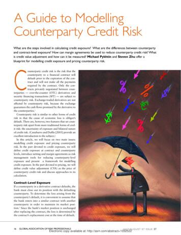
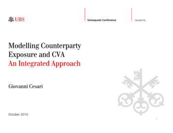
4.1Portfolio CharacteristicsThe analysis presented in this section is based on a large portfolio of over-thecounter derivatives including positions in interest rate swaps and credit defaultswaps with approximately 4,800 counterparties. We focus on two cases, the largest220 and largest 410 counterparties as ranked by exposure (EPE); these two casesaccount for more than 95% and 99% of total portfolio exposure respectively.Figures 1 and 2 present exposure concentration reports, giving the number of effective counterparties among the largest 220 and 410 counterparties respectively.10The effective number of counterparties for the entire portfolio in shown in Figure3. As can be seen in these figures the choice of largest 220 and 410 counterpartiesis justified as the number of effective counterparties for the entire portfolio is 31in each case.Effective Counterparty Number30Number of eff CP252015effective counterparty number1050122446688110132154176198220Figure 1: Effective number of counterparties for the largest 220 counterparties.The exposure simulation uses M 1000 and M 2000 market scenarios, whilethe systematic credit risk factor is discretized with N 1000, N 2000 andN 5000 using the method described above. For CVaR calculations, we employthe 95% and 99% confidence levels11 .The ranges of individual counterparty exposures are plotted in figure 4. The 95thand 5th percentiles of the exposure distribution are given as a percentage of the10Counterparty exposures (EPEs) are sorted in decreasing order. Let wn be the nth largestexposure; then the Herfindahl index of the N largest exposures is defined as:HN PNn 1P2wn/( Nn 12wn )The effective number of counterparties among the N largest counterparties with respect to total 1portfolio exposures is HN.11Although α 99.9% is the most commonly used confidence level in practice, we chose the95% and 99% as our results are best depicted by our choice of N in the coming section.11
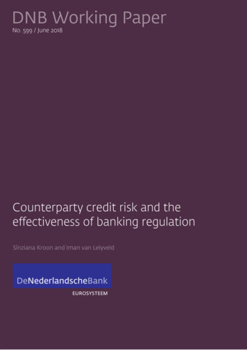
Effective Counterparty Number35effective counterparty number30Number of eff CP252015105014182123164205246287328369410Figure 2: Effective number of counterparties for the largest 410 counterparties.Effective Counterparty Number35effective counterparty number30Number of eff CP252015105016001200180024003000360042004794Figure 3: Effective number of counterparties for the entire portfolio.mean exposure for each counterparty. The volatility of the counterparty exposuretends to increase as the the mean exposure of the respective counterparties decreases. In other words, counterparties with higher mean exposure tend to be lessvolatile compared to counterparties with lower mean exposure. Given the abovecharacteristics, we would expect that wrong-way risk could have an importantimpact on portfolio risk, and that the contribution of idiosyncratic risk will alsobe significant. The distribution of the total portfolio exposures from the exposuresimulation is given in Figure 5. The histogram shows that the portfolio exposuredistribution is both leptokurtic and highly skewed. It is important to employsuch highly skewed with very fat tail exposure distribution to ensure the properconservatism of our method in practice.12
Percentiles of the distribution of exposures for individual counterparties450%95% percentile trendMean exposure5% percentile trend400%% of mean 240Counterparty280320360400Figure 4: 5% and 95% percentiles of the exposure distributions of individual counterparties, expressed as a percentage of counterparty mean exposure (Here counterpartiesare sorted in order of decreasing mean exposure).90Base Case8070Frequency605040302010060708090100Exposure (% base case mean)110120130Figure 5: Histogram of total portfolio exposures from the exposure simulation.4.2Numerical ResultsTo assess the severity of the worst-case joint distribution, and to determine the degree of conservativeness in earlier methods, we compare risk measures calculatedusing the worst-case joint distribution to those computed based on the stresstesting algorithm presented in Garcia-Cespedes et al. [2010] and Rosen and Saunders [2010]. In this method, exposure scenarios are sorted in an economicallymeaningful way, and then a two-dimensional copula is applied to simulate thejoint distribution of exposures (from the discrete distribution defined by the exposure scenarios) and the systematic credit factor. The algorithm is efficient, andpreserves the (simulated) joint distribution of the exposures. Here, we apply aGaussian copula, and sort exposure scenarios by the value of total portfolio exposure (this intuitive sorting method has proved to be conservative in many tests,13
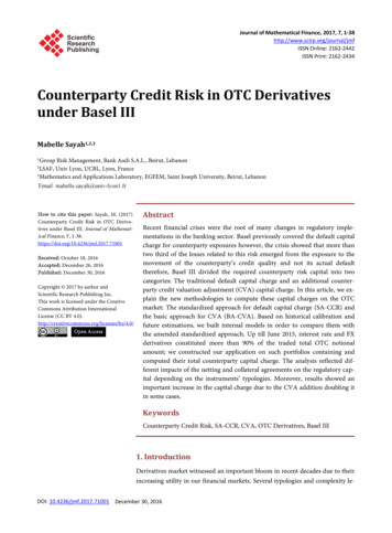
Case IM N O(106 )α0.950.99Case IIM N O(106 )α0.950.99Case IIIM N O(107 )α0.950.99M 1000 market scenariosmin(CVaRsys /CVaRwcc )52.2%51.8%N 1000 credit scenariosmax(CVaRsys /CVaRwcc )95.1%95.9%M 2000 market scenariosmin(CVaRsys /CVaRwcc )50.3%49.6%N 2000 credit scenariosmax(CVaRsys /CVaRwcc )96.9%96.6%M 2000 market scenariosmin(CVaRsys /CVaRwcc )44.8%44.1%N 5000 credit scenariosmax(CVaRsys /CVaRwcc )96.4%97.1%Table 1: Minimum and maximum of ratio of systematic CVaR using the Gaussian copula algorithm to systematicCVaR using the worst-case joint distribution for the largest 220 counterparties at 95% and 99% confidence level.Case IM N O(106 )α0.950.99Case IIM N O(106 )α0.950.99Case IIIM N O(107 )α0.950.99M 1000 market scenariosmin(CVaRtot /CVaRwcc )52.2%51.6%N 1000 credit scenariosmax(CVaRtot /CVaRwcc )96.8%96.5%M 2000 market scenariosmin(CVaRtot /CVaRwcc )49.6%48.9%N 2000 credit scenariosmax(CVaRtot /CVaRwcc )97.2%97.4%M 2000 market scenariosmin(CVaRtot /CVaRwcc )45.8%44.7%N 5000 credit scenariosmax(CVaRtot /CVaRwcc )98.1%98.2%Table 2: Minimum and maximum ratio of CVaR for total losses using the Gaussian copula algorithm to CVaR fortotal losses using the worst-case joint distribution for the largest 410 counterparties at 95% and 99% confidencelevel.conducted in Rosen and Saunders [2010]). For each level of correlation in theGaussian copula, we calculate the ratio of risk (as measured by 95% and 99%CVaR) estimated using the sorting method to risk, which in turn, is estimatedusing the worst-case loss distribution.We present the results of three discretizations of the worst-case joint distribution.The first case employs M 1,000 market scenarios and N 1,000 credit scenarios; the second case doubles the market and credit scenarios. In third case we use2,000 market scenarios and 5,000 credit scenarios. Note that the first and secondcases I and II yield a discretized worst-case distribution of O(106 ) while the thirdcase’s output is of O(107 ).Figure 6 shows the graph of the ratio of systematic CVaR using the Gaussiancopula algorithm described in Rosen and Saunders [2010] to systematic CVaR us14
Case ICase IICas
tions to counterparty credit risk are emphasized, and they include assessing wrong-way risk in the credit valuation adjustment, and counterparty credit risk measurement. Lastly a detailed application of the algorithm for coun-terparty risk measurement to a real portfolio case is also presented in this paper.