Transcription
Department of PhysicsUmeå UniversityFebruary 4, 2017Credit Risk Modeling and ImplementationReport 1.2Johan Gunnars (jogu0081@student.umu.se)Master’s Thesis in Engineering Physics, 30.0 credits.Supervisor: Oskar Janson (oskar.janson@cinnober.com)Examiner: Markus Ådahl (markus.adahl@umu.se)
Johan Gunnars (jogu0081@student.umu.se)February 4, 2017AbstractThe financial crisis and the bankruptcy of Lehman Brothers in 2008 lead toharder regulations for the banking industry which included larger capital reserves for the banks. One of the parts that contributed to this increased capitalreserve was the the credit valuation adjustment capital charge which can beexplained as the market value of the counterparty default risk. The purpose ofthe credit valuation adjustment capital charge is to capitalize the risk of futurechanges in the market value of the counterparty default risk.One financial contract that had a key role in the financial crisis was the creditdefault swap. A credit default swap involves three different parts, a contractseller, a contract buyer and a reference entity. The credit default swap can beseen as an insurance against a credit event, a default for example of the reference entity.This thesis focuses on the study and calculation of the credit valuation adjustment of credit default swaps. The credit valuation adjustment on a creditdefault swap can be implemented with two different assumptions. In the firstcase, the seller (buyer) of the contract is assumed to be default risk free andthen only the buyer (seller) contributes to the default risk. In the second case,both the seller and the buyer of the contract is assumed to be default risky andtherefore, both parts contributes to the default risk.i
Johan Gunnars (jogu0081@student.umu.se)February 4, 2017SammanfattningFinanskrisen och Lehman Brothers konkurs 2008 ledde till hårdare regleringarför banksektorn som bland annat innefattade krav på större kapitalreserver förbankerna. En del som bidrog till denna ökning av kapitalreserverna var kreditvärdighetsjusteringens kapitalkrav som kan förklaras som marknadsvärdet avmotpartsrisken. Syftet med kreditvärdighetsjusteringens kapitalkrav är att kapitalisera risken för framtida förändringar i marknadsvärdet av motpartsrisken.Ett derivat som hade en nyckelroll under finanskrisen var kreditswappen. Enkreditswap innefattar tre parter, en säljare, en köpare och ett referensföretag.Kreditswappen kan ses som en försäkring mot en kredithändelse, till exempelen konkurs på referensföretaget.Detta arbete fokuserar på studier och beräkningar av kreditvärdesjusteringenpå kreditswappar. Kreditvärdesjusteringen på en kreditswap kan implementerasmed två olika antaganden. I det första fallet antas säljaren (köparen) vara riskfri och då bidrar bara köparen (säljaren) till konkursrisken. I det andra falletantas både säljaren och köparen bidra till konkursrisken.ii
Johan Gunnars (jogu0081@student.umu.se)February 4, 2017Contents1 Introduction1.1 Background . . . . . . . . . . . . . .1.2 Counterparty Credit Risk . . . . . .1.3 Over-The-Counter . . . . . . . . . .1.4 Credit Default Swap . . . . . . . . .1.4.1 Credit event . . . . . . . . . .1.4.2 Settlement . . . . . . . . . .1.4.3 The Usage of CDS Contracts1.5 Regulations . . . . . . . . . . . . . .1.6 Credit Valuation Adjustment . . . .1.7 Right and Wrong Way Risk . . . . .111122334552 Theory2.1 Credit Default Swap . . . . . . . . .2.1.1 Premium Leg . . . . . . . . .2.1.2 Protection leg (Payment Leg)2.1.3 Credit Default Swap Payoff .2.2 Hazard and Survival Function . . . .2.3 Credit Valuation Adjustment . . . .2.3.1 Unilateral CVA for CDS . . .2.3.2 Bilateral CVA for CDS . . .2.3.3 Default Correlation . . . . . .2.3.4 CIR Intensity Model . . .66677899910113 Method3.1 Construction of Hazard Rate and Survival Probability Curve3.1.1 Premium Leg . . . . . . . . . . . . . . . . . . . . . . .3.1.2 Protection leg . . . . . . . . . . . . . . . . . . . . . . .3.1.3 Bootstrapping hazard rate . . . . . . . . . . . . . . . .3.1.4 Survival probability . . . . . . . . . . . . . . . . . . .3.2 CVA for CDS . . . . . . . . . . . . . . . . . . . . . . . . . . .3.2.1 Calibration of CIR Process . . . . . . . . . . . . .3.2.2 CIR Simulation . . . . . . . . . . . . . . . . . . . .3.2.3 Conditional Survival Probability . . . . . . . . . . . .3.2.4 Fractional Fast Fourier Transform . . . . . . . . . . .3.2.5 Conditional Gaussian Copula Function . . . . . . . . .1212121213141415161717194 Results214.1 Survival Curve Construction from Market Spreads . . . . . . . . 214.2 Unilateral CVA . . . . . . . . . . . . . . . . . . . . . . . . . . . . 234.3 Bilateral CVA . . . . . . . . . . . . . . . . . . . . . . . . . . . . . 265 Discussion5.1 Survival Curve Construction from Market Spreads5.2 Unilateral and Bilateral CVA . . . . . . . . . . . .5.3 Future Work . . . . . . . . . . . . . . . . . . . . .5.3.1 Adjoint Algorithmic Differentiation. . . . .5.3.2 Interest Rate Swaps . . . . . . . . . . . . .iii.303030313131
Johan Gunnars (jogu0081@student.umu.se)5.3.35.3.4February 4, 2017Collateralized CVA . . . . . . . . . . . . . . . . . . . . . .Calibration of Intensity Process Parameters . . . . . . . .A AppendixA.1 Derivation of Conditional Copula .A.2 CDS Input Data . . . . . . . . . .A.3 CVA Input Parameters . . . . . . .A.4 Unilateral CVA Simulation ResultsA.5 Simulation Verification Results . .A.5.1 Risk Free Investor . . . . .A.5.2 All Parts Risky . . . . . . .iv.31313434353737404043
Johan Gunnars (jogu0081@student.umu.se)11.1February 4, 2017IntroductionBackgroundCinnober FT is a developer of financial systems for clearing of financial transactions. The primary function of the clearing house is to eliminate counterpartyrisk between the two parties of a trade. The trades most commonly handledby a clearing house are those created on exchanges. The clearing house insertsitself as the counterparty to both the seller and the buyer. The clearing housecalculates a risk margin value that both parts of the trade have to post as collateral while the trade is being cleared. If one part involved in the trade failsto fulfill their obligation, the clearing house can take this collateral and settlewith the other part of the trade.However, if you are trading outside the exchange, on the so called over thecounter market (OTC), a clearing houses may not be involved. This means thatyou are directly exposed to the credit risk of your counterparty.The goal of the thesis is to investigate and implement credit risk models. Thecompleted implementation will rely on a sound theoretical framework complemented with recognized best practices and be possible to run on top of actualmarket data such as CDS spreads.1.2Counterparty Credit RiskThe financial risk is normally divided into smaller parts. One important part isthe counterparty credit risk or just counterparty risk, but to be able to explaincounterparty risk, there are two other parts of the financial risk that have to beexplained.Credit risk can be explained as the risk that a debtor is unable or unwilling tomake a payment to fulfill contractual obligations. This is generally known as adefault.Market risk is the risk of losses in positions arising from movements in marketprices. If it is linear, it arises from an exposure to the movements of underlyingvariables such as stock prices and credit spreads. This risk can be eliminatedby entering into an offsetting contract.Counterparty risk represents a combination of market risk, which defines theexposure and the credit risk, which defines the credit quality of the counterpart,(Gregory, 2012).Counterparty risk is of major importance in over the counter derivatives becausethe counterparty risk is mitigated in exchange traded derivatives, (MosegardSvendsen, 2014).1.3Over-The-CounterThe over-the-counter (OTC) market is the off-exchange market and the largestdifference from the exchange market is that the participants of a trade aredirectly exposed to the credit risk, the risk of a default of the counterpart. Whentrading on the exchange, a clearing house act as a middle part and eliminatesthe credit risk and make sure that the trade goes through by taking collateral,a fee depending on how risky every part of the trade is.1
Johan Gunnars (jogu0081@student.umu.se)1.4February 4, 2017Credit Default SwapThe credit default swap (CDS) is an agreement between two parties to exchangethe credit risk of a reference entity, (Beinstein and Scott, 2006). The CDScan easiest be explained as an insurance but there are differences between aninsurance and a CDS. The largest difference is that the CDS buyer does notneed to own what he/she insure. This means that by buying a CDS, you couldinsure someone else’s property.The buyer of the contract, pays regular payments to the seller of the contract.In the case of a credit event for the reference entity, the payments stop and theseller of the CDS pays a large amount to the buyer. If the contract expires, theseller has received regularly payments and does not need to pay anything back.Figure 1: The credit default swap consists of three parts, the protection buyer,the protection seller and a reference entity.1.4.1Credit eventThe trigger of the CDS contract is called a credit event. These are a few possiblecredit events, explained by (Beinstein and Scott, 2006): Bankruptcy: Includes insolvency, creditor arrangements and appointment of administrators. Failure to pay: When a payment on one or more obligations fails afterany grace period. Restructuring: Refers to a change in the agreement between the reference entity and the holder of the obligation due to the deterioration increditworthiness or financial condition to the reference entity. This withrespect to reduction of interest or principal, postponement of payment ofinterest or principal, change of currency and contractual subordination.2
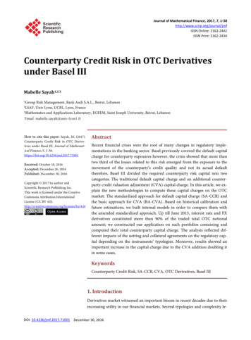
Johan Gunnars (jogu0081@student.umu.se)1.4.2February 4, 2017SettlementLet us assume that an investor is exposed to an entity through a bond andwants to hedge the default risk of the entity. Then the investor can buy a CDSwith this entity as the reference.If the reference entity defaults before the maturity of the CDS, then the investor of the CDS will receive a single default payment from the seller of thecontract. This is called settlement. The settlement is usually physical or in cash.If the settlement is physical, the investor deliver the bond to the seller of theCDS in exchange for a payment equal to the face value of the bond.If the settlement is in cash, the investor receives a payment of the differencebetween the face value and the market value of the bond.1.4.3The Usage of CDS ContractsThere are several different application for credit default swaps.Let us assume that there are three companies, named A,B and C.In this first example, company A is lending company B 1 million and willreturn 10% of interest per year. Company A wants to insure the loan and buysa CDS from company C with company B as reference entity. Company A pays1% of the loan to company C in exchange for an insurance against a default ofcompany B, see Figure 2. In the event of a default of company B, company Cwill compensate company A for the loss. If company B would have defaultedwithout the CDS, company A would not get the money back.Figure 2: Example 1 to the left and example 2 to the right.In this second example, company A suspects that company C will default in thenear future and buys a CDS from company B with company C as the referenceentity. Company A pays periodic payments to company B and receives a default3
Johan Gunnars (jogu0081@student.umu.se)February 4, 2017payment in the case of a default of company C, see Figure 2. This is the samething as buying an insurance on someone else’s car and hoping that the car willsuffer an accident.In this last example, company A is a pension fund that wants to invest theirmoney. The problem is that they can only lend their money to someone witha very high credit rating. Let us assume that company B wants to borrow themoney from company A but the credit rating of company B is too low. Inthis case, company A can buy a CDS from company C with company B asthe reference entity. Lets assume that the credit rating for company C is thehighest possible. Then company A would lend their money to company B andcompany C will compensate company A in the case of a default of companyB, see Figure 3. The result of this example is that company A will lend theirmoney to company B which now have the credit rating of company C.Figure 3: Example 3.1.5RegulationsToo big to fail is a concept that can be explained as when a company is soessential to the economy in the world, the government will bail them out in caseof bankruptcy to prevent a global economic disaster. Trading with one of thesecompanies was considered risk free but the latest financial crisis in 2008 and thebankruptcy of Lehman Brothers showed that no investments are risk free.The Basel accords were constructed to reduce the banks’ market and creditrisk exposure. The framework of Basel I mainly focuses on credit risk. Basel IIwas more risk aware and was based on three pillars. Minimum capital requirements, supervisory review and the market discipline. Basel II was implementedin the middle of the financial crisis at 2008 but before it was completely implemented, Basel III began to develop. This lead to the fact that Basel II neverreached its full potential.Basel III was implemented after the financial crisis and focuses mainly on the4
Johan Gunnars (jogu0081@student.umu.se)February 4, 2017risk of a bank run and requires larger capital reserves by the banks. One ofthe parts that were added to the total counterpart credit risk capital charge inBasel III is the credit valuation adjustment capital charge (CVA capital charge).(Norman and Chen, 2013).The purpose of the CVA capital charge is to capitalize the risk of future changesin CVA. Every new accord comes with harder regulations and that trend willprobably continue.1.6Credit Valuation AdjustmentCVA is the difference between the risk free portfolio value and the true portfoliovalue that includes the possibility of a counterpart default. In other words, CVAis the market value of counterpart credit risk, (Pykhtin and Zhu, 2007).1.7Right and Wrong Way RiskRight and wrong way risk is a concept that comprises a correlation between thedefault risk of a counterpart and the value of the underlying contract. Wrongway risk occurs in the case of a positive correlation and right way risk with anegative correlation.When the default risk of the counterpart increases at the same time as the valueof the contract increases, the wrong way risk will increase the CVA. The rightway risk is the opposite, with an increasing default risk and a decreasing valueof the contract, the CVA will decrease.One example of wrong way risk is then a company sells a put option, the rightbut not the obligation, to sell the companies own stock. When the stock price decreases, the value of the put option increases. When the stock price decreases,the default risk of the company increases. (Hoffman, 2011) and (Milwidsky,2011).5
Johan Gunnars (jogu0081@student.umu.se)2February 4, 2017TheoryThis section consists of three parts. The first part describes the parts of thecredit default swap and the valuation of the contract. The second part describesthe theory behind the hazard rate and the corresponding survival probability.The final part gives the theory behind bilateral credit valuation adjustment.This involves simulation of an intensity model, correlation of defaults and valuation of the bilateral credit valuation adjustment.2.1Credit Default SwapThe theory in this section is based on (Brigo and Mercurio, 2006).A credit event of the referent will from now be denoted as a default and thethree parts of the contract will be denoted as: 0 Investor, the part that calculates the CVA 1 Reference entity 2 Counterpart, the part that the CVA is calculated onThe default time is denoted by τi where the index i 0,1,2 represents thedifferent parts of the contract. The protection buyer pays regular payments atthe rate of S, the spread, at the predetermined times Ta 1 , Ta 2 , ., Tb until thecontract expires or until a default of the reference entity occurs.In exchange, the protection buyer receives a payment of the loss given default(LGD) on the notional at a default of the reference entity. The LGD can obtaina maximum value of 1 when the full notional is paid and a minimum value of 0when nothing is paid.2.1.1Premium LegThe value of the premium leg is the present value of the payments that is madeby the protection buyer, (Cojocaru and Militaru, 2014).With the assumption that the stochastic discount factor D(s, t) is independentof the default time τ1 for all 0 s t, the value of the premium leg at time 0of the CDS can be defined as: PremiumLega,b (S) E D(0, τ1 )(τ1 Tγ(τ1 ) 1 )S1{Ta τ1 Tb } bX E D(0, Ti )αi S1{τ1 Ti }i a 1ZTbP (0, t)(τ1 Tγ(τ1 ) 1 )Q(τ1 [t, t dt)) St Ta SbXP (0, Ti )αi Q(τ1 Ti )i a 1ZTb SP (0, t)(τ1 Tγ(τ1 ) 1 )dt Q(τ1 t)t Ta SbXi a 16P (0, Ti )αi Q(τ1 Ti )(1)
Johan Gunnars (jogu0081@student.umu.se)February 4, 2017where αi is the year fraction between Ti 1 and Ti , Tγ(τ1 ) 1 is the last paymentdate before τ1 , P (0, t) is the zero coupon bond observed from the market thatdiscounts the payments back from time t to 0 and Q(τ1 T ) is the survivalprobability. τ1 represents the default time of the reference entity.The integral term represent the accrued premium which is the fraction of thepremium that has accrued from the preceding payment date up to the defaulttime and the summation term represents the discounted payments, (O’Kaneand Turnbull, 2003).2.1.2Protection leg (Payment Leg)The value of the protection leg is the present value of the amount that the protection buyer receives in the case of a default of the reference entity, (Cojocaruand Militaru, 2014).With the assumption that the default time τ1 and the interest rates are independent, the value of the protection leg at time 0 of the CDS can be definedas: ProtecLega,b (LGD) E 1{Ta τ1 Tb } D(0, τ1 )LGDZ Tb LGDP (0, t)Q(τ1 [t, t dt))(2)t TaZ Tb LGDP (0, t)dt Q(τ1 t))t Ta2.1.3Credit Default Swap PayoffBy again assuming that the default time and the interest rates are independentand that the recovery rate is deterministic, the value of a CDS contract to theseller at time t is given by:CDSa,b (t; S) PremiumLega,b (t; S) ProtecLega,b (t; S)(3)(Milwidsky, 2011). To obtain the value of the CDS to the protection buyer, thesigns in front of the legs is switched.Given a CDS contract at time 0 for a default of the reference entity betweentime Ta and Tb , with the periodic premium rate S1 and the loss given defaultLGD1 , the value of the CDS to the protection seller is given by:" ZTbP (0, t)(t Tγ(t) 1 )dt Q(τ1 t)CDSa,b (0, S1 , LGD1 ) S1 t Ta#bX P (0, Ti )αi Q(τ1 Ti )(4)i a 1"Z#TbP (0, t)dt Q(τ1 t) LGD1t Tawhere γ(t) is the first payment in period Tj following time t.We now denoteNPV(Tj , Tb ) : CDSa,b (Tj , S, LGD1 )7(5)
Johan Gunnars (jogu0081@student.umu.se)February 4, 2017the residual NPV of a receiver CDS between the times Ta and Tb evaluated atTj , where Ta Tj Tb . NPV is the net present value.Equation (5) can be written on the same form as Equation (4) but for evaluationat time Tj :NPV(Tj , Tb ) CDSa,b (Tj , S1 , LGD1 )( 1τ1 Tj" ZS1 TbP (Tj , t)(t Tγ(t) 1 )dt Q(τ1 t FTj )max{Ta ,Tj } bX P (Tj , Ti )αi Q(τ1 Ti FTj ) (6)i max{a,j} 1"Z#)TbP (Tj , t)dt Q(τ1 t FTj ) LGD1max{Ta ,Tj }where evaluation is conditioned on the information that is available to the market at time Tj , FTj . (Brigo and Capponi, 2008).2.2Hazard and Survival FunctionThe theory in this section is based on (Rodriguez, 2010).Let us assume that T is a continuous random variable, f (t) is the pdf, F (t) P r {T t} is the cdf which gives the probability of an event has occurred byduration t. The survival function is defined as the complement of the cdf:Z Q(t) P r {T t} 1 F (t) f (x)dx(7)tThe survival function gives the probability that a default has not occurred untiltime t. The hazard rate is the instantaneous rate of default and can be definedas:P r {t T t dt T t}(8)λ(t) limdt 0dtThe numerator gives the conditional probability of default in the interval [t, t dt)given that a default has not already occurred, and the denominator is the widthof the interval. By taking the limit of the expression and letting dt go to zero,the result obtained is the instantaneous rate of default, or the hazard rate.According to (Schönbucher, 2003), the hazard rate can be rewritten as:λ(t) f (t)Q(t)(9)This formula means that the default rate at time t is equal to the probability density function at t divided by the survival probability until time t. Bycombining Equation (7) and Equation (9), the hazard rate can be expressed as:dlogQ(t)(10)dtIf we integrate the expression from 0 to t, the survival probability at time t canbe written as a function of the hazard rates up to time t: Z t Q(t) exp λ(x)dx(11)λ(t) 08
Johan Gunnars (jogu0081@student.umu.se)February 4, 2017The integral is the cumulative hazard function and it can be viewed as the sumof the risks from time 0 to t:Z tΛ(t) λ(x)dx.(12)0Given the hazard rates, the survival function can be calculated and given thesurvival function, the hazard rates can be calculated. The survival functiongives the curve with the probability of default at different times. The hazardrate is the short time probability of default.2.3Credit Valuation AdjustmentThe theory in this section is based on (Brigo and Capponi, 2008).The unilateral credit valuation adjustment (UCVA) can be explained as thedifference in the price for a contract with a default risk free counterpart andthat with a default risky counterpart. The bilateral credit valuation adjustment(BCVA) can be explained as the difference in the price for a contract with adefault risk free investor and counterpart and the price of the contract with adefault risky investor and counterpart, (Hoffman, 2011). The CVA can be seenas the price of the default risk.Let us now define long and short position for the CVA calculation. Long: Calculated from the buyer, on the seller of the CDS. Short: Calculated from the seller, on the buyer of the CDS.2.3.1Unilateral CVA for CDSThe unilateral credit valuation adjustment for the short position is given by:UCVAa,b (t, S, LGD1,2 ) LGD2 Et 1{t τ2 T } P (t, τ2 ) NPV(τ2 )] (13)and for the long position:UCVAa,b (t, S, LGD1,2 ) LGD2 Et 1{t τ2 T } P (t, τ2 ) NPV(τ2 )] (14)From Equation (13), (14) and (6), it is clear that the only terms that are leftto calculate are:1τ1 τ2 Q(τ1 t Fτ2 )(15)2.3.2Bilateral CVA for CDSLet us define the following events: A {τ0 τ2 T } Investor defaults before counterpart, both defaultsbefore the maturity of the contract. B {τ0 T τ2 } Investor defaults before the maturity of the contract,the counterpart defaults after the maturity.9
Johan Gunnars (jogu0081@student.umu.se)February 4, 2017 C {τ2 τ0 T } Counterpart defaults before the investor, both defaultsbefore the maturity of the contract. D {τ2 T τ0 } Counterpart defaults before the maturity of thecontract, the investor defaults after the maturity.The bilateral credit valuation adjustment for the short position is given by:BCVAa,b (t, S, LGD0,1,2 ) LGD2 Et {1C D P (t, τ2 ) [ NPV(τ2 )] }(16) LGD0 Et {1A B P (t, τ0 ) [ NPV(τ0 )] }and for the long position:BCVAa,b (t, S, LGD0,1,2 ) LGD2 Et {1C D P (t, τ2 ) [ NPV(τ2 )] }(17) LGD0 Et {1A B P (t, τ0 ) [ NPV(τ0 )] }From Equation (16), (17) and (6), is is clear that the only terms that are leftto calculate are:1C D 1τ1 τ2 Q(τ1 t Fτ2 )(18)and1A B 1τ1 τ0 Q(τ1 t Fτ0 )(19)The big advantage for BCVA against Unilateral CVA is that BCVA is symmetric. The BCVA of the investor is minus the BCVA for the counterpart,(Hoffman, 2011).2.3.3Default CorrelationLet us assume that the defaults are correlated between the parts of the contract.The dependence is modeled by using a trivariate Gaussian copula function. Theexponential random variables that characterizes the default times are modeledwith the dependence function. The default intensities λi for the parts of thecontract are assumed to be independent of each other. By assuming that thecumulative intensities are strictly positive, Λi will be invertible. The defaulttimes τi can be defined asτi Λ 1i (ξi ), i 0, 1, 2(20)where ξi is a standard unit-mean exponential random variable. From the properties of exponential random variables follows thatUi 1 exp( ξi )(21)are uniform [0, 1] randomly distributed which are correlated through a Gaussiantrivariate copulaCR (u0 , u1 , u2 ) Q(U0 u0 , U1 u1 , U2 u2 )where R is a correlation matrix.10(22)
Johan Gunnars (jogu0081@student.umu.se)2.3.4February 4, 2017CIR Intensity ModelThe stochastic intensity model that we chose for simulation of the paths for thethree parties of the contract isλj (t) yj (t) ψj (t; βj ), t 0, j 0, 1, 2(23)where ψ is a deterministic function that depends on the parameter vector βjand is integrable on closed intervals. yj is assumed to be a Cox Ingersoll Ross(CIR) process that is given byqdyj (t) κj (µj yj (t))dt νj yj (t)dZj (t), j 0, 1, 2(24)The parameter vectors are βj (κj , µj , νj , yj (0)) where all components are positive deterministic constants. Zj is assumed to be standard Brownian motionthat are independent. One note is that the Feller condition 2κj µj νj2 thatprevent the CIR process for attending a zero value is not imposed. Instead aconstraint is imposed on the deterministic shift ψ that makes it strictly positiveand because the CIR process cannot become negative, the CIR process becomes strictly positive and nonzero.We also define the following integrated quantities that will be used laterZ tZ tZ tΛj (t) λj (s)ds, Yj (t) yj (s)ds, Ψj (t; βj ) ψj (s; βj )ds(25)00011
Johan Gunnars (jogu0081@student.umu.se)3February 4, 2017MethodThis section describes the method for the implementation. The first part ofthe implementation consists of constructing the hazard rate curve and the corresponding survival probability curve. The second part of the implementationconsists of the calculation of the bilateral credit valuation adjustment for acredit default swap.3.1Construction of Hazard Rate and Survival ProbabilityCurveThe theory that the method in this section is based on comes from (O’Kaneand Turnbull, 2003). To be able to calculate the hazard rate curve, there are afew input parameters that are necessary. The first are the risk-free zero rates,that are used for discounting payments. The second parameter is the recoveryrate R and the third parameter is the market spreads S for a set of tenors. Themodel that is selected for the calculation of the hazard rates is the JPMorganmodel. This model assumes that the default occurs midway during the period.The accrued payment is made at the end of the period.From the zero rates, the zero curve can be calculated by interpolating the zerorates and then calculate the discount factors that are needed.For the 4Y data, the quarterly discount factors are given so we just need todo a interpolation to obtain the monthly discount factors (because the modelcalculates the payment leg monthly). This interpolation is done linearly.3.1.1Premium LegLets assume that there are n 1, ., N contractual payment dates t1 , ., tN ,where tN is the maturity date. The premium leg is defined in Equation (1) andby using the approximation given by (O’Kane and Turnbull, 2003), the premiumleg can be written as:PremiumLeg(tV , S) S(tV , tn )NXP (TV , tn )αn Q(tV , tn )n 1NS(tV , tn ) XP (tV , tn )αn (Q(tV , tn 1 ) Q(tV , tn )) 2n 1 (26)NS(tV , tn ) XP (tV , tn )αn (Q(tV , tn 1 ) Q(tV , tn ))2n 1where tV is the time of evaluation and accrued premium is assumed. S(tV , tn ) isthe spread for the corresponding payment date tn Equation (26) is the expressionthat we are going to use for the calculation of the hazard rates and the survivalprobabilities.3.1.2Protection legThe protection leg is defined in Equation (2) and by using the approximation in(O’Kane and Turnbull, 2003), we will get the following expression for calculation12
Johan Gunnars (jogu0081@student.umu.se)February 4, 2017of the protection leg:ProtecLeg(tV , R) (1 R)MX tNP (tV , tm )(Q(tV , tm 1 ) Q(tV , tm ))(27)m 1where M is a finite number of discrete points per year. This expression will beused for calculation of the hazard rates and the survival probabilities.3.1.3Bootstrapping hazard rateThe spread is assumed to be break even which implies that the payment leg isequal to the premium leg. By setting Equation (26) equal to Equation (27),rearranging some terms and rewrite the probabilities in terms of the hazardrates, we get the following expression under the assumptions that the CDS havequarterly payments and monthly discretization:S(tv , tv 1Y ) Xe λn τn e λn τn 3P (tv , tn )αn1 R2n 3,6,9,12 12XP (tv , tm )(e λm τm 1 e λm τm(28))m 1where τn and τm are discretization factors:τ0 0.0, τ1 0.0833, τ2 0.167, ., τ12 1.00(29)The only unknown terms in Equation (28) is the hazard rate which can be solvedfor the first period by usin
Counterparty risk represents a combination of market risk, which de nes the exposure and the credit risk, which de nes the credit quality of the counterpart, (Gregory, 2012). Counterparty risk is of major importance in over the counter derivatives because the counterparty risk is mitigated in exchange traded derivatives, (Mosegard Svendsen, 2014).