Transcription
Journal of Mathematical Finance, 2017, 7, 1-38http://www.scirp.org/journal/jmfISSN Online: 2162-2442ISSN Print: 2162-2434Counterparty Credit Risk in OTC Derivativesunder Basel IIIMabelle Sayah1,2,3Group Risk Management, Bank Audi S.A.L., Beirut, LebanonLSAF, Univ Lyon, UCBL, Lyon, France3Mathematics and Applications Laboratory, EGFEM, Saint Joseph University, Beirut, Lebanon12How to cite this paper: Sayah, M. (2017)Counterparty Credit Risk in OTC Derivatives under Basel III. Journal of Mathematical Finance, 7, d: October 18, 2016Accepted: December 26, 2016Published: December 30, 2016Copyright 2017 by author andScientific Research Publishing Inc.This work is licensed under the CreativeCommons Attribution InternationalLicense (CC BY en AccessAbstractRecent financial crises were the root of many changes in regulatory implementations in the banking sector. Basel previously covered the default capitalcharge for counterparty exposures however, the crisis showed that more thantwo third of the losses related to this risk emerged from the exposure to themovement of the counterparty’s credit quality and not its actual defaulttherefore, Basel III divided the required counterparty risk capital into twocategories: The traditional default capital charge and an additional counterparty credit valuation adjustment (CVA) capital charge. In this article, we explain the new methodologies to compute these capital charges on the OTCmarket: The standardized approach for default capital charge (SA-CCR) andthe basic approach for CVA (BA-CVA). Based on historical calibration andfuture estimations, we built internal models in order to compare them withthe amended standardized approach. Up till June 2015, interest rate and FXderivatives constituted more than 90% of the traded total OTC notionalamount; we constructed our application on such portfolios containing andcomputed their total counterparty capital charge. The analysis reflected different impacts of the netting and collateral agreements on the regulatory capital depending on the instruments’ typologies. Moreover, results showed animportant increase in the capital charge due to the CVA addition doubling itin some cases.KeywordsCounterparty Credit Risk, SA-CCR, CVA, OTC Derivatives, Basel III1. IntroductionDerivatives market witnessed an important bloom in recent decades due to theirincreasing utility in our financial markets. Several typologies and complexity leDOI: 10.4236/jmf.2017.71001 December 30, 2016
M. Sayahvels of such instruments are used either in a regulated exchange traded manneror in an over the counter fashion. Instruments could be swaps, options, futures,forwards. Exchange traded activity started in 1970 following certain rules and“standardized” formats whereas over the counter (OTC) market came in 1990 asan “irregular” market with various customizable trades; therefore it is a morerisk vulnerable environment. OTC market has a larger volume due to the higherprofit margin and wider bid-ask spreads. Trying to reduce the risk on the OTCmarket, clearing houses were created in order to give all the counterparties aguarantee not to have any open positions and to force applications of the agreedupon rules.Derivatives hold several types of risks such as market, liquidity and credit,however the credit risk in such instruments is not the typical credit risk that weencounter when passing a loan; it is the counterparty credit risk. The counterparty credit risk differs from the traditional credit risk by two points: The bilateral risk profile and the variation of the exposure depending on market andcounterparty behavior. Counterparty credit risk is the risk taking into accountthe exposure of the financial institution to the counterparty if this latter defaultsor has its credit quality devaluated. Recent crises emphasized the faulty practicesregarding the OTC derivatives capital charge computation from a counterpartycredit risk point of view: Starting with the collapse of Lehman Brothers and several near and full collapses of banks all over the United States, United Kingdomand Europe, the counterparty risk gained now the same importance as the majorwell-known risks (market, liquidity, operational ). Counterparty credit risk hasgained importance making it a central need in several areas of the bankingworkflow: Pricing OTC products, computing the capital charges, managing exposures to different counterparties and finally stating the conditions of a certaindeal concerning the initial margin or collateral Basel II had implemented methods to compute the default capital charge of the counterparty credit risk beardin derivatives however in the subprime crisis two thirds of the losses did not result from such category of counterparty risk. A new risk source was highlighted:the risk resulting from the credit valuation of the counterparty noted the creditvaluation adjustment risk (CVA). In this paper our aim is to describe the currentOTC market, to briefly note the previously applied regulatory methods for thecounterparty credit risk then to explain and apply the new methods in order tocompute the capital requirements on typical portfolios. The paper proposes alsoan internal approach to compute the same figures based on historical behaviorand future market experts’ estimations. Section I introduces the counterpartycredit risk, Section II details the default capital charge whereas Section III detailsthe CVA risk capital charge. Section IV presents the application of such techniques compared to internal approaches on sample portfolios and finally SectionV concludes on the results.2. Counterparty Credit RiskCounterparty Credit risk is a major risk faced on the OTC market. It covers two2
M. Sayahfacts: the defaults of the counterparty or the decrease in its credit quality as described in [1]. In both scenarios, the bank would try to replace the instrumentheld or re-evaluate its worthiness. In order to compute this “replacement cost”and “potential future exposure” different factors are involved such as: Mark-tomarket exposure, liquidity risk following a counterparty’s default, operationalrisk as in the process of managing the positions after a change had occurred oreven in managing the margins or collaterals of a certain agreement and finallylegal risk related to enforcement for the application of the deals conditions. Asthe use of derivatives has grown, especially on the OTC market, regulators arecontinuously trying to implement new approaches that reflect as adequately aspossible the counterparty risk englobed by these instruments and thereforemaking their approaches more and more sophisticated, see [2].2.1. Transition to BaselIn an attempt of improving capital framework for OTC derivatives under BaselIII method presented in [3], several reforms were put in place: Wrong way Risk is more adequately evaluated by not taking recoveries in theloss given default (LGD) computation (the amount lost in case of the counterparty’s default). The computation of the portfolio exposure is required to take into account astressed period values (in LGD calibration). New method for collateralized transactions evaluations to capture the exposure over a full year of inception. Standards for initial margining have been strengthen. The asset value correlation parameter was increased by 25% to reflect thecorrelations between financial institutions raising the risk weights.Another important change in Basel III is the addition of a credit valuationadjustment (CVA) capital charge to capture the risk of mark to market losseson the expected counterparty credit risk, this is amply described in [4]. Totallosses from CVA were double the losses from defaults (66% from CVA andonly 33% of the losses are due to defaults). The CVA capital charge is expectedto double the capital charge for derivatives however, banks are not going to beasked to put any additional CVA charge if the derivatives are centrally cleared:This is an incentive to clear through a central counterparty clearing house(CCP).2.2. Default Capital Charge ComputationAll banks are required to hold capital against the variability in the market valueof their OTC instruments: They need to capitalize for default risk. As it is wellknown for Basel amended approaches two possibilities are entitled: A standardized approach and an internal model implementation. In the following, we aregoing to discuss briefly the characteristics and method scheme of each of thesemethods in order to apply them in the following part of this work and comparetheir figures.3
M. Sayah2.2.1. Standardized Counterparty Credit Risk Approach (SA-CCR)SA-CCR is the new standardized approach for computing default counterpartycredit risk presented in the BCBS document [5]. It was presented and revised byApril 2014 and is in order to be implemented by January 2017. Different papersdescribed this method such as [6], in our work we try to summarize and apply iton different portfolios under different conditions in order to understand the behavior of this practice.Main objectives of this method implementation were to be: Suitable to be applied on different kinds and specifications of derivativestransactions Easy and simple implementation techniques Better than the methods that preceded More risk sensitivity reflectionComputing the capital charge is our main aim and this figure is given by:Default Counterparty Capital Charge Exposure at default Risk weight 8% (1)Where the SA-CCR EAD (Exposure at default) is our key figure, the riskweight is amended by Basel and the 8% reflects the pillar 1 obligation.Computing the EAD would need to be held on each netting set level on ahedging set basis:EAD 1.4 ( RC PFE )(2)where RC is the replacement cost and PFE the potential future exposure.The concept of Equation (2) is referring to is the fact that the exposure to aninstrument is the sum of its present value and the future potential values. Thealpha factor is added as an insurance to cover the risk and the value of alpha iscalibrated based on several internally generated models (seen in previous counterparty credit risk models), therefore this coefficient is kept constant all throughthe computation.Hedging sets are defined as follows (details in pages 12 - 13 of document [5]):1) Interest rate: a hedging set is defined for one same currency further dividedinto maturities, long and short positions fully offset within maturity categories, across maturity categories partial offset is recognized2) Foreign exchange: same currency pairs form same hedging sets, full offset isonly permitted within a same pair3) Credit derivatives and Equity derivatives: in these two categories each assetclass forms a hedging set, full offset is permitted for a same entity (index orname) whereas partial offset between derivatives is applied when referring todifferent entities4) Commodity derivatives: four hedging sets: energy, metals, agriculture andothers. No offset among these categories. In a same hedging set, full offset forsame commodity is permitted and partial offset is applied when handlingdifferent commodities.The EAD formula changes in case the trade is margined or un-margined: If margined: RC represents the exposure if the counterparty defaults at time4
M. Sayaht 0 assuming the close-out does not take time and PFE is the change invalue during the period between the default and the deployment of the collateral. If un-margined: RC is the present exposure and PFE is the potential increasein exposure over a one-year time horizon.Replacement CostThe RC is computed following two formulas: if the trade is margined or not(more details in [7], pp. 4-7.For un-margined transactions: RC max ( 0;V C )(3)where V is the current market value of the derivatives and C is the net haircutcollateral held. Not having any margin, at time t 0 the replacement costwould depend on two possible outcomes: the instrument’s value is in our favoror not. If the value of the instrument is higher than the collateral a default of thecounterpart would result in a loss equal to V-C the value of the instrument minus the collateral value, if not, no loss is included: which explains the RC formulation in the un-margined case.For margined transactions:RC max ( 0;V C ; TH MTA NICA )(4)where TH is the positive threshold before the counterparty send the bank collateral, MTA is the minimum transfer amount applicable to the counterparty andNICA any collateral posted by the counterparty minus the one posted by thebank (net value). In this case the margin should be taken into account for thecomputation of the replacement cost: if the value of the instrument is inferior tothe value of the collateral and the collateral posted by the bank is inferior to theone posted by the counterparty, the loss will be null. However, if any of the previously denoted figures is positive the replacement cost will be equal to it: if theposted collateral is more than the collateral of the counterparty or if the value ofthe instrument is higher than the total collateral the bank would have to coverthese differences as a replacement cost.Potential Future ExposurePFE is given by:PFE multiplier Add On Aggregatewhere the multiplier recognizes excess of collateral and negative mark-tomarket, and the add-ons are calculated for each asset class.Computing the multiplier also detailed in [7], with a floor of 5% is computedas follows: V Cmultiplier min 1; floor (1 floor ) exp 21floorAddon aggregate (){} The multiplier formula is built in a way to account for over-collaterization:The multiplier is normally at 1 however, if the bank chooses to over-collaterizethe instrument they are holding, this multiplier will be inferior to 1 therefore5
M. Sayahgiving the bank the advantage of their extra-safety arrangement.And the add-on computation follows these steps:1) Define the transaction primary risk factor.2) Allocate it to an asset class: Interest rate (IR), Foreign exchange (FX), equity,credit or commodity3) Compute the adjusted notional amount (for IR and credit duration is included).4) Get the maturity factor (whether margined or not).5) Multiply the supervisory delta by the adjusted notional ( or 1 if long orshort).6) Multiply it by the given supervisory factor to reflect volatility.7) Aggregate by hedging sets and asset-class level.For more details on the specific computation of the Add-on for each assetclass, please refer to the Basel document [7].The SA-CCR add-on computation method is based on a set of assumptions inorder to result in the previously cited formulas. These assumptions are the following: All trades are at the money (MtM 0). The banks neither hold nor post collateral. No cash flows are present before the one-year horizon. The evolution process of instruments follows a Brownian motion with zerodrift and fixed volatility.We note the important impact of the maturity factor on the computation: thislatter depends on the portfolio: margined or not. If the portfolio is un-margined,the maturity factor (MF) applied is equal to:MFun margined min (1year, Maturity )1year(5)However, if the portfolio is margined, MF depends on the remargining frequency. Basel amends a certain margin period of risk (MPOR) depending on thecharacteristics of the deals considered, this margin represents the closing timebetween the default of the counterparty and the margin payment. This concept isdescribed in [5].MFmargined 3 MPOR2250(6)where MPOR is defined by the frequency: for daily re-margining MPOR isequivalent to 10. The general formula for an N remargining per day frequency is:MPOR 10 N 1(7)A daily re-margin is the most conservative, therefore we chose this frequencyas a base of our application portfolios (in Section II.7).However, we note that the 3 2 multiplier maintained by Basel in order toapproach the EE of a margined transactions to the one of an un-marginedtransaction for MPOR (reflected in [7]) is resulting in double accounting for theshock (1.5 1.4).6
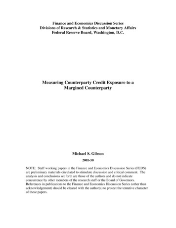
M. SayahSeveral comments were presented to try and remove this multiplier, such asthe comments by Deutche bank, however, the multiplier remains present in thefinalized version of the method.A brief description of the SA-CCR mentioned above is shown in Figure 1.2.2.2. Internal Model Method (IMM)As the habit went, all internal models to be applied for banks should be acceptedby the supervisor entitled for this bank (the national regulator). The bank in ourcase study is free to choose to model internally the EAD for the OTC derivatives.Having this in mind, Basel implemented in its third version [3] requirementsthat should be respected in order to get approval for the proposed internal model. Please note that due to several different approaches that could be consideredin the internal model approach, in a consultative document, refer to [8], Baselproposed to floor the IMM capital charge to a certain percentage of the SA-CCRcapital charge or better yet remove the IMM as an approved method to computeand report capital charges under the counterparty credit risk. However, all OTCinstruments that were not included in the internal model or that could not assume approval to be globalized under the internal model should be treatedthrough the standardized approach. We shall briefly describe the requirementsfor the EAD internal model but we note that these requirements are required ona permanent basis and continuous check-ups will be put in place in order to ensure the fully compliance to these rules all through the period of application ofthe chosen internal model.In an attempt to make this more pleasant for readers and easier to discuss theconditions for the implementation of an internal model will be represented asFigure 1. SA-CCR capital charge computation process.7
M. Sayahbullet points under each categories of requirements: The model should specify a forecasting distribution for changes in marketvalue such as interest rate or foreign exchange rate. For margined counterparties, the model should also capture the future behavior of the collateral in question. Note that no particular form of model isrequired. Determining the default capital charge should be based on the greater computation using: once the current market data to calibrate the projection models and once a stressed calibration. In both cases the time frame should bethree years and in the stressed conditions it should cover a stressed period inbetween (three years containing a stress among them). The computation will follow these given steps: the Exposure at Default(EAD) is the product of a previously calibrated (and negotiated) α factorand the Effective Expected Positive Exposure:EAD α EEPE(8)Effective Expected Positive Exposure (EEPE) relies on internal model to predict counterparty exposures, typically simulating underlying market risk factorsout to long horizons and revaluating counterparty exposures at future datesalong the paths simulated, it is the weighted average of the Effective ExpectedExposure (EEE). EEPEmin (1year,maturity ) k 1EEE k k(9)The EEE is the increasing function of the Expected Exposure (EE): thisamends a more restrictive approach, once an exposure is hit the method doesnot permit a decrease in the exposure for future dates.EEE k max ( EEE k 1 , EE k )(10)where k tk tk 1 and EE k being the average exposure at future date kacross possible future values of relevant market risk factors, and alpha set for 1.4however a discussion permitting lower or greater alpha is possible (floored at1.2). A more detailed look on these formulas is clearly presented in Pykhtin’s article [9]. The exposure should not only be limited for a given time horizon (ex: oneyear), it should cover the entire life of the portfolio (the OTC portfolio). Again for margined transactions, the internal model should account for there-margining period, the mark-to-market valuation and a sets of floors set forthe time horizons of deals. An independent management unit responsible for calculating and makingcalls for margin should be put in place. The bank must present: adequate documentation for the counterparty creditrisk (CCR) management process, validation of the models, organizationalapproval, accurate reporting and reflective results. Before starting to use the model, a bank should calculate it for at least oneyear before implementation in order to have a set of observed outcomes of8
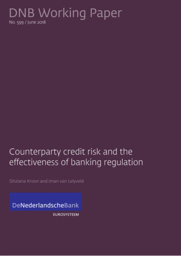
M. Sayahthe chosen approach.In the rest of this paper, we will choose for each case a given forecasting modelin order to project the risk factors (interest rate and foreign exchange risk), calibrate it twice: once on a normal market and once in stress conditions, computethe EE and going up the formulas recover the EAD for the instrument in question in the both cases, the maximum EAD will be our IMM exposure at default.We note that the calibration, the re-evaluation and the models chosen for theIMM could change the capital charge amended by such approaches: the relativevariability for IMM appears to be considerable between banks. Basel committeeconducted an exercise in an attempt to compare the outcome of such modelsbetween banks and recommend a best practice for the IMM in the counterpartycredit risk framework, this exercise can be found in [10].3. CVA Capital Charge ComputationThe CVA capital charge applies to all derivative transactions that are subject tothe risk that a counterparty could default. However, the scope of applicationdoes not include derivatives cleared through a clearing (central) counterparty. Italso encompasses securities financing transactions that are fair-valued by a bankfor accounting purposes. CVA risk could be seen as a strong link between thecounterparty and the market risk however it is by nature more complex thanmarket risk on the trading book leading to different frameworks and choicesabout precise implementation. Reference [11] discusses this issue precisely. Recent Basel approaches amended two frameworks for the computation of thiscapital charge: The Fundamental Review of the Trading Book CVA framework(FRTB-CVA) and a Basic CVA approach (BA-CVA) as shown in Figure 2. Under the FRTB concept, banks are asked to compute the CVA sensitivities requiring the simulation of all exposures to a large panel of market risk factors. Thisprocedure is very demanding, therefore some banks are enable to cover this calculation and therefore the basic approach presented in [12] is an option for thesereasons. In February 2016, a QIS was sent by Basel to be calculated by banks on avoluntarily basis in order to measure the impact of these different approaches onthe computation of the CVA capital charge, QIS found in [13].Figure 2. CVA capital charge computation methodologies.9
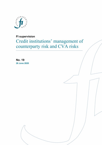
M. Sayah3.1. Standardized CVA (SA-CVA, FRTB)Eligibility Criteria:1) Ability to compute CVA sensitivities.2) Methodology to approximate credit spreads for all counterparties (includingilliquid ones).3) Existence of an independent CVA risk management function.Eligible hedges: Single-name instruments, proxy hedges and market riskhedges.CVA calculation:At least a monthly computation is entitled: For each counterparty (even if only one derivative is included).The SA-CVA capital is the sum of delta and Vega risks. Each one of these categories are divided into sub-categories depending on the risk types as shown below in Figure 3. For each type, a certain methodology is used to bucket the assets and to compute their sensitivity.For each risk type in both categories we compute (refer to BCBS (2015) p.16-25): Sensitivity of the aggregate CVA Sensitivities of all eligible hedges Compute weighted sensitivities: Risk weights are given by Basel for each risktype. The net weighted sensitivity is the sum of the CVA weighted sensitivities andtheir hedges. Within each bucket, weighted sensitivities are aggregated to form the bucket’s cc. Across buckets computation results in the total capital (detailed descriptionin [14]).3.2. Advanced Internal Model Method IMM-CVA FRTBThe use of this method is conditioned upon approval of supervisor’s authority.Briefly citing the conditions: regular back testing, a trial period, expected shortfall approach, 97.5 confidence level, cover delta and vega risks, stressed periodFigure 3. Standardized CVA categorization.10
M. Sayahcalibration. The methodology is to compute internally the CVA expected shortfall (netted assumptions) and then to compute this figure for each asset types:interest rate, FX, credit spread, equity and commodities in order to sum all ofthem and get the gross expected shortfall. The average of the two expectedshortfalls is considered and a regressive formula is put in place in order to compute the required capital charge.3.3. Basic CVA (BA-CVA)The basic CVA approach is for banks that are not able to compute the CVA sensitivity or does not have the approval of their authorities to use the FRTB-CVAintroduced in [12]. However, this approach is known to be very demanding andvery conservative in terms of risk weights placed by Basel.Before detailing the computation of the capital charge it is important to citevery briefly the eligible hedges in this framework: single-name CDS that references the counterparty directly, or references an entity legally attached to it orreferences an entity that belongs to the same sector and region of this counterparty; single-name contingent CDS and index CDS.The basic CVA capital charge is given by the sum of the spread capital( Kspread ) and the expected exposure capital ( K EE ) :(11)K K spread K EECVAThe formulation of the capital charge is intuitive because the CVA is the risk abank is facing in case of a fluctuation in the credit quality of the counterpartytherefore the two main factors are the credit quality represented by K spread andthe expected exposure amount parallel to this change: K exposure . Differentiationin computation apply if the portfolio is hedged or not (hedging the CVA risk ornot). Considering that no hedging strategies were put in place for hedging thiskind of risk, which is the case for the majority of small and medium banks having the CVA as a relatively new capital charge computation, we will apply thefollowing formula:2 2 ρ Sc 1 ρ c unhedgedK spread() Sc2c(12)where Sc is the supervisory expected shortfall of CVA of counterparty c andρ is the supervisory correlation between the credit spread of a counterpartyand the systematic factor set to ρ 50% .The second term of Equation (8) is given by a simple scaling of K spread :unhedgedK EE 0.5 K spread(13)Therefore the computation is held in the Sc term:Sc RWb( c )α M NS EAD NSNS c(14)α is non-other than the α 1.4 discussed earlier, EAD are the EAD internally computed earlier on a netting set level, M NS is the effective maturity of the11
M. Sayahnetting set and RWb ( c ) is the risk weight set by Basel for the risk bucket b( c ) .The different weights are shown in Basel paper [12].4. Application4.1. Data UsedIn the following, we chose to work on three different portfolios composed eachtime of one unique instrument: an interest rate swap, an FX forward and a FXplain vanilla call respectively. No netting is considered and no collateral normargin agreements are added in this first step.In each scenario, we computed the capital charge of the portfolio for differentmaturities of the instrument (going from 6 months to 5 years) in order to see theprogression in time of the capital charge (in standardized or internal approaches).The choice was made due to different causes: To cover several asset classes. To study differences between instruments with or without optionality. The interest rate segment accounts for the majority of OTC derivatives activity and represented around 80% of the global OTC derivatives market byJune 2015. Foreign exchange derivatives make up the second largest segment of theglobal OTC derivatives market with around 13% of the market by mid-2015,and FX forwards make up half of the notional amount outstanding in thisasset class.We detail the three considered portfolio in this section:IR swaps: We start by considering a portfolio containing one interest rateswap denoted in USD: one floating leg and one fixed leg of 100 USD as notionalwith semi-annual payments. The fixed coupon rate is defined in a way for thepresent MtM of the swap to be null. We will consider different versions of thisportfolio by changing the maturity of the swap: from a 6-month interest rateswap to a five-year swap.FX forward: We consider a portfolio containing one FX forward USD-EUR.The forward rate is computed in such way that the present MtM is null. As wedid earlier, we will consider different cases of this portfolio by changing the maturity of the forward: from a 6 month FX forward to a five year FX forward.Plain vanilla option: We consider a portfolio with a single FX plain vanillacall (USD/EUR), long position, with maturities going from 6 months up till 5years, a notional of 100 EUR, a strike price of 1.4 (the actual spot is 1.0963). TheMtM of the call is not null and it is priced using the Black and Scholes formulawith the market implied volatility.The data used are fetched from Bloomberg platform: (see Appendix 2 for theplots) USD swap curve, EURO swap curve and the FX spot rate (USD-EUR). For each swap curve the observed tenors are 1 month up till 50 years. Daily frequency.12
M. Sayah Historical observed dates: since end of April 2004 until end of April 2007. Swap curve number of observations: 1536 per tenor (112,128 observations). FX curve: 1565 observations.4.2. Capital Charge Computation4.2.1. Default Capital ChargeConsidering a risk weight of 100% and the pillar 1 factor as 8%, by multiplyingthe obtained EAD by these two components we would be able to
however the credit risk in such instruments is not the typical credit risk that we encounter when passing a loan it is the counterparty credit risk. The counter; - party credit risk differs from the traditional credit risk by two points: bila- The teral risk profile and the variation of the exposure depending on market and counterparty behavior.