Transcription
Swissquote ConferenceLausanneModelling CounterpartyExposure and CVAAn Integrated ApproachGiovanni CesariOctober 20101
Basic Concepts CVA Computation Underlying Models Modelling Framework: AMC CVA: C‐CDS approach Next StepsBasic ConceptsSection 12
What is Counterparty Credit Exposure?Exposure to loss due to failure by a counterparty to perform Counterparty Credit Exposure: exposure to loss due to failure by a counterparty to perform Counterparty risk is at the root of traditional banking Historically, the first form of financial instruments were bonds Value driven by the perceived credit worthiness Financial transactions typically involves cash flows to other institutions or individual If any of these counterparty should fail to fulfill their obligation there will be a replacementcost incurred Take‐and‐hold exposure Lending products – loans, commitments Trading products – OTC products / SFTsWe focus on OTC!3
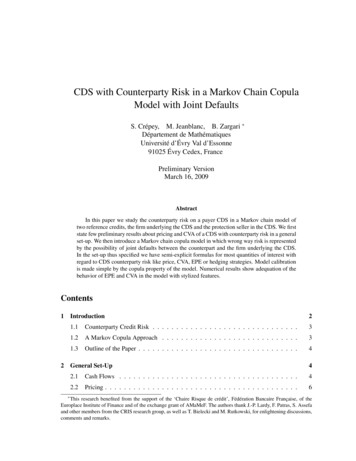
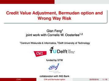
Typical Counterparty Exposure Risk MeasuresPFE and EPE are the key statistical measures Compute price distributionsat different times in thefuture Statistical measures are thencalculated on this pricedistribution Potential Future Exposure (PFE),usually a quantile measure at97.5% or 99% Expected Positive Exposure (EPE),the mean of the positive part ofthe distributionFrequencyMean of thedistributionEPEStandard Deviation ofthe distributionProbabilitydistributionPFE2.5%0Trade value Mean ExposureWe will see that these measures have different meanings depending on the context4
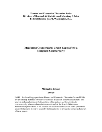
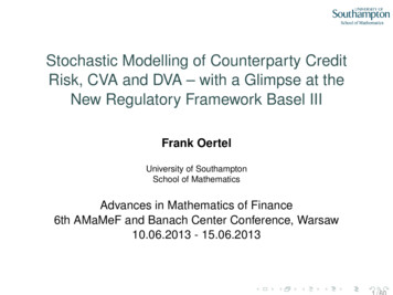
Computing Exposure by SimulationExample: Vanilla SwapPFEEPEPortfolioValuePastPresentFuture5
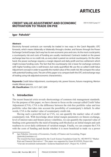
What is CVA?Counterparty exposure from a pricing perspective CVA ‐ Credit Value Adjustment It is the price of counterparty credit exposure It is an adjustment to the price of a derivative to take into account counterparty creditexposure It is not the only adjustment that we need to make however Risk FreeDerivative RiskyDerivative CVA6
Fair Value of a Financial InstrumentThere are several adjustments required to adjust Mark‐To‐Market valueFVA Cost of FundingModel specific adjustmentCVA, DVA: Cpty and Bank DefaultTV RV – CVA DVA ‐ FVA7
Basic Concepts CVA Computation Underlying Models Modelling Framework: AMC CVA: C‐CDS approach Next StepsCVA ComputationSection 28
CVA ComputationCVA is a pricing measure: some details In case of default at time we pay the positive part of the value of the portfolio Max[V,0]Positive part ofportfolio valueRecovery onportfolioWe pay if a defaultoccurs is the default timet T (maturity) Pricing is done via Risk Neutral ValuationIntegral: wesum over allpossible timeintervalsExpectation is inthe measure NNumeraire:Risk neutraldiscounting9
CVA ComputationThe EPE x Spread approach We can now discretize the interval to compute the integral and assume spreadconstant over the interval: this approach has some deficienciesExposure at Default Protection Leg ofForward starting CDSModified EPEExpectation in the measure NExposure at de10Discounted exposure
CVA vs Counterparty Exposure: Fundamental DifferencesBoth compute price distributions at different times in the future, but Counterparty Exposure Statistical measures Potential Future Exposure (PFE), usually aquantile measure at 97.5% or 99% Expected Positive Exposure (EPE), the mean ofthe positive part of the distribution PFE is used against limits EPE is used for RWA and capital CVA CVA is the cost of buying protection on thecounterparty that pays the portfolio value in case ofdefault Expected Positive Exposure (EPE), the expected valueunder the risk neutral measure It is now a considerable part of the PnL of anyfinancial institution Needs to be hedged Enters in VaR11
Basic Concepts CVA Computation Underlying Models Modelling Framework: AMC CVA: C‐CDS approach Next StepsUnderlying ModelsSection 312
Set‐Up Computation of counterparty credit exposure Interest Rate Swaps and Cross Currency Swapsand of CVA for portfolio of OTC transactions, Exotic interest rate products, CMS, steepenerincluding both vanillas and exotics Exotic options on equity, FX, commodities Credit Default Swaps, CDO Models need to be Scenario consistent across products Powerful enough to deal with exotic transactions Powerful enough to be used for pricing andhedging: CVA computation The framework needs to be Flexible enough to deal with different types ofproducts, booked and priced in different system Models and framework need to be able to Take into account collateral and cost of collateral Possibly be extended to consider other aspects e.g.cost of funding13
Choice of ModelsUnderlying simulations Risk Models Pricing Models: TV Physical measure Pricing measure (risk neutral) Simulations are not (necessarily) used for pricing Simulations are used for pricing (Monte Carlo pricing) Calibration with historical values Calibration with market instruments Conservative measures Focus on accuracy Portfolio view Each product can be priced in isolation Scenario consistency across asset classes Hedging Future price distributions Very large book of transactions CVA Models Scenario consistency Pricing measure Future price distributions Simulations are used for pricing Portfolio view Calibration with market instruments Very large book of transactions Focus on accuracy Hedging14
Model Roadmap15
Basic Concepts CVA Computation Underlying Models Modelling Framework: AMC CVA: C‐CDS approach Other ApplicationsModelling Framework: AMCSection 416
Typical Counterparty Exposure ProfileVanilla Interest Rate Swap Consider an interest rate swap We receive the 6 month Libor rate on a notionalof 100 million We pay a fixed rate equal to the par 10 yearswap rate The swap contract has zero value atinception As time passes and market conditionchanges accordingly If the swap rate decreases, the transaction willbe out of the money If the swap rate increases, the transaction willbe in the money to us and if the counterpartydefaults, this is a mark‐to‐market credit loss tous As time passes, the amount of paymentsdecreases and hence we have lessexposure17
Recipe for Computing Credit ExposureAt the highest level, all credit exposure systems Scenario Generation Generate the scenario from a model, calibratedusing the latest market data Pricing Price the instruments on each scenario in thefuture Aggregation Add up all the prices of each product at eachscenario and each time point18
Challenge to the Monte Carlo ApproachProducts with embedded optionality Now suppose that we have the option tocancel a trade at no cost We are long callability Conversely, we are short callability if the otherside can cancel a trade at no cost We would walk away from the trade ifthe mark‐to‐market value of the swapplus the option is negative The profile is similar to a normal swap, exceptthe starting point is the value of the option From a computational point of view,there is a fundamental differencebetween vanilla swap and this embeddedoptionality Vanilla swaps can be priced off the yield curve,while the Bermudan swap requires a model tovalue19
Other Challenges The Monte Carlo framework seems to give a good implementation recipe. In practice,there are issues that needs to be addressed The generation of correlated scenarios is not trivial, potentially thousands of differentrisk factors driving the dynamics of different and often complex products The scenarios have to be consistent across all systems to build a counterparty view This is the key issue with the current generation of front office systems, it is not designed with this inmind Need the same family of underlying models for all product types, same numeraire Pricing functions developed in various libraries are not necessary designed to beintegrated in a counterparty exposure framework. This has implications from both a software and architecture prospective Not all products can be computed in analytic form. Most exotics are priced either usingPDE or Monte Carlo approachesNeed of an alternative approach!20
American Monte CarloAMC neatly resolves the problem of pricing and exposure calculation in one step The basic idea is to approach thecounterparty exposure as a pricingproblem and thus use pricing algorithms American Monte Carlo algorithm Instead of building a price moving forward intime Starts from maturity, where the value of theproduct is known and goes backward AMC is used in general for products withCallability Products whose value depends a strategy whichcan only be determined by only knowing futurestates of the world The benefit of this approach is that a pricedistribution is also provided The algorithm is generic an hence onlythe payoff is required21
The Credit Exposure ProblemDefining a product with early exercise features Suppose that we have a generic product with early‐exercise features, which we denoteby P. The holder is entitled to cash flows X Apart from X, P also gives the holder the replace, at specific points in time, to a post‐exercise portfolio Q.Write the set of possible exercise time as If exercise happens at maturity, then the value of the trade is provided by P and is embodied inNumeraireExpectation in theN‐measure The optimality criterion by which the holder chooses the optimal time to exercise the option will bedescribed later22
The Credit Exposure ProblemAssuming optimal exercise time, the valuation can be given in two parts The price distribution of product P can be given asOptimal Exercise Time The value prior to exercise is given byNumerairePre‐ExerciseCash Flow ValuesPost‐ExerciseCash Flow Values23
American Monte CarloThe valuation is done via a recursive procedureContinuation Value There are several approaches thatmay be employed to compute theoptimal exercise decision rule This involves estimating at each timestep at the expected value of notexercising, conditional on the currentvalue and the value of theobservablesInductive stepVP(i)Decision whether toExercise or notV(i) The key is to estimate the conditionalexpectations of the product and thepost exercise portfolioProduct Value?V(i 1)VQ(i)TiPost ExercisePortfolio ValueTi 124
American Monte CarloThe conditional expectation is estimated using a regression The only remaining question is on how toestimate the conditional expectation We construct an estimator using a regressionon polynomial functions on the observables Regressing the discounted future values against thecurrent observables There are many possible basis functions tochoose from, our implementation usespolynomials The choice of basis function have very limited impacton the quality of result The choice of the observable itself is importantObservables E[Current values] f(Future values)25
Valuation ErrorsAMC is an approximation The price distribution computed via AMCyields an estimate of the true price Errors can come from the following Choice of observables – As observables are theparameters driving prices, the wrong choice couldlead to unreliable result Regression error – The type of regression functionand their order could impact the result Bundling – The size of bundling can influenceresult The graph on the right shows the differencein profile for a vanilla interest rate swap We pay floating and receive fixed The EPE is near identical The lower PFE is subject to more numerical noise26
High Level Architecture DescriptionThe key idea is to homogenize the booking descriptions and models for the purpose ofportfolio evaluation In order to compute exposure at portfoliolevel, it is necessary to collect all tradesthat are booked on different pricingsystems Easily compute exposure of trades that usuallyare described via termsheet Decouple trade description from implementationof analytics Bring trades from existing booking systems into asingle unified booking representation27
Example 1A Physically Settled SwaptionNotional 10 mm USD;Schedule From 2009/03/31 to 2019/03/31 Every 3 Months;Swap Receive (Notional * IR:USD6M * 0.25) USD on Schedule;Swap Pay (Notional * 3% * 0.25) USD on Schedule;Long callable on 2013/03/31 into swap;Cash SettledPhysicalSettled28
Example 2SteepenerNotional 10 mm EUR;Schedule from 2009/05/09 to 2029/11/29 Every 6 Months;Steepener Receive Notional * (4.84% 2*Max(0,(1.33%-(EUR 20y – EUR2y)))on Schedule;Steepener Pay (Notional * EUR 6m) on Schedule;Long callable every 1 year from 2010/05/21 to 2029/11/21;29
Basic Concepts CVA Computation Underlying Models Modelling Framework: AMC CVA: C‐CDS approach Next StepsCVA: C‐CDS ApproachSection 530
CVA ComputationDynamic EPE ‐ the C‐CDS approach CVA can be computed as “EPE x Spread” In reality, EPE is itself risky: underlying portfolio may have interest rate, FX, credit, equity,inflation risk Portfolio effects might further complicate this: correlation risk EPE is always positive part of portfolio: embedded optionality volatility risk It can be useful to have a view on how CVA can could change during the life of the trade Right‐Way / Wrong –Way effects might alter CVA pricing and risk / hedgingAll these effects are difficult to capture through the traditional “EPE x Spread” approach31
CVA ComputationDynamic EPE ‐ The C‐CDS approach Rather than seeing CVA as a reserve, see it as the value of a derivative We call this derivative a C‐CDS ‐ Contingent Credit Default Swap Contingent, because value paid upon default of the counterparty is dependent on thevalue of an underlying transaction/portfolio CVA C‐CDS value Valuation of CVA through a C‐CDS approach requires Monte Carlo valuation techniques This allows to directly control Right/Wrong‐Way effects linking underlying risk drivers todefault of the counterparty32
CVA ComputationDynamic EPE ‐ The C‐CDS approach The valuation can then be performed byMonte Carlo technique using the followingpayoff0 Suppose we have the full simulation of theunderlying portfolio value Simulate the default time of the counterpartyat each path and then take the value of theportfolio at that timeX It is possible for the counterparty not to defaultduring the life of the trade Take expectation across all paths to computethe C‐CDS price from the payoff The price of the C‐CDS is the CVA33
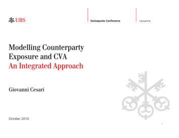
C‐CDSExistence of the price distribution means that we can have a long term view of the riskdue to CVA As an illustration, consider a 10 year USDswap on a notional of 1000m USD Receive 3 month USD Libor fixed in advance Pay a fixed coupon equal to today’s par Assume the counterparty’s CDS curve isflat 130 bps The initial point is equal to today’s CVA ataround 8.4m USD, The underlying interest rate and spreadrisk means that the CVA could reach up to22m USD at 97.5% confidence level34
Wrong Way – Right Way RiskAdvantages of using a C‐CDS approach Using a C‐CDS approach it is possible to include in the simulation of counterpartydefaults correlation with other risk factors In the case of credit derivatives (e.g. CDS, or CDO) it is straightforward to includecorrelation between defaults of the underlying and of the counterparty Correlation with other risk factors can be more challenging35
Basic Concepts CVA Computation Underlying Models Modelling Framework: AMC CVA: C‐CDS approach Next StepsNext StepsSection 636
Open Questions and Challenges (From a Quant Perspective) CVA vs. counterparty exposure Do we want different models for CVA (pricing) and counterparty exposure (control)? Physical vs risk neutral measure Models What is the level of accuracy required (e.g. interest rate exotics)? What is the required level of consistency with other pricing systems (e.g. CDO)? Can we use the AMC approach for all products? Hedging Which sensitivities are needed, how often should they be computed? Collateral, Close‐out and CVA Should we take into account close‐out risk? How should we model collateral – which curve should be used? Cost of collateral cost of funding and DVA Should we recognize DVA? How do we include cost of funding?37
Need of having accurate models across portfoliosManaging Banks Scarce Resources Resource allocation has to be performedon a portfolio basisBalance sheetRWA/capital Models need to be flexible and powerful enoughto price accurately transactions in futurescenariosDVACounterparty limitallocation A time‐zero pricing view is not enough A “risk” view is not accurate enough We have all the ingredients to be able tocompute different risk measures across allasset classes and portfoliosEngineClientfranchise(client creditsCVAMarket spreadFundingand liquiditymanagementCollateral management andcredit mitigantsOperatingcostper trade38
DISCLAIMERBy accepting this document, the recipient agrees to be bound by the following obligations and limitations.This presentation has been prepared by UBS AG and/or its subsidiaries, branches or affiliates (together, “UBS”) for the exclusive use of the party to whom UBS delivers this presentation (the “Recipient”). The information in this presentation has been obtained from the Recipient andother publicly available sources and has not been independently verified by UBS or any of its directors, officers, employees, agents, representatives or advisers or any other person. No representation, warranty or undertaking, express or implied, is or will be given by UBS or itsdirectors, officers, employees and/or agents as to or in relation to the accuracy, completeness, reliability or sufficiency of the information contained in this presentation or as to the reasonableness of any assumption contained therein, and to the maximum extent permitted bylaw and except in the case of fraud, UBS and each of its directors, officers, employees and agents expressly disclaim any liability which may arise from this presentation and any errors contained therein and/or omissions therefrom or from any use of the contents of thispresentation.This presentation should not be regarded by the Recipient as a substitute for the exercise of its own judgment and the Recipient is expected to rely on its own due diligence if it wishes to proceed further.The valuations, projections, estimates, forecasts, targets, prospects, returns and/or opinions contained herein involve elements of subjective judgment and analysis. Any opinions expressed in this material are subject to change without notice and may differ or be contrary to opinionsexpressed by other business areas or groups of UBS as a result of using different assumptions and criteria. This presentation may contain forward-looking statements. UBS gives no undertaking and is under no obligation to update these forward-looking statements for eventsor circumstances that occur subsequent to the date of this presentation or to update or keep current any of the information contained herein and this presentation is not a representation by UBS that it will do so. Any estimates or projections as to events that may occur in thefuture (including projections of revenue, expense, net income and stock performance) are based upon the best judgment of UBS from the information provided by the Recipient and other publicly available information as of the date of this presentation. Any statements,estimates, projections or other pricing are accurate only as at the date of this presentation. There is no guarantee that any of these estimates or projections will be achieved. Actual results will vary from the projections and such variations may be material.Nothing contained herein is, or shall be relied upon as, a promise or representation as to the past or future. This presentation speaks as at the date hereof (unless an earlier date is otherwise indicated in the presentation) and in giving this presentation, no obligation is undertakenand nor is any representation or undertaking given by any person to provide the recipient with additional information or to update, revise or reaffirm the information contained in this presentation or to correct any inaccuracies therein which may become apparent.This presentation has been prepared solely for informational purposes and is not to be construed as a solicitation, invitation or an offer by UBS or any of its directors, officers, employees or agents to buy or sell any securities or related financial instruments or any of the assets,business or undertakings described herein. The Recipient should not construe the contents of this presentation as legal, tax, accounting or investment advice or a personal recommendation. The Recipient should consult its own counsel, tax and financial advisers as to legal andrelated matters concerning any transaction described herein. This presentation does not purport to be all-inclusive or to contain all of the information that the Recipient may require. No investment, divestment or other financial decisions or actions should be based solely on theinformation in this presentation.This presentation has been prepared on a confidential basis solely for the use and benefit of the Recipient. Distribution of this presentation to any person other than the Recipient and those persons retained to advise the Recipient, who agree to maintain the confidentiality of thismaterial and be bound by the limitations outlined herein, is unauthorized. This material must not be copied, reproduced, published, distributed, passed on or disclosed (in whole or in part) to any other person or used for any other purpose at any time without the prior writtenconsent of UBS; save that the Recipient and any of its employees, representatives, or other agents may disclose to any and all persons, without limitation of any kind, the tax treatment and tax structure of the transaction and all materials of any kind (including opinions or othertax analyses) that are provided to the Recipient relating to such tax treatment and tax structure.By accepting this presentation, the Recipient acknowledges and agrees that UBS is acting, and will at all times act, as an independent contractor on an arm’s length basis and is not acting, and will not act, in any other capacity, including in a fiduciary capacity, with respect to theRecipient. UBS may only be regarded by you as acting on your behalf as financial adviser or otherwise following the execution of appropriate documentation between us on mutually satisfactory terms.UBS may from time to time, as principal or agent, be involved in a wide range of commercial banking and investment banking activities globally (including investment advisory, asset management, research, securities issuance, trading (customer and proprietary) and brokerage), havelong or short positions in, or may trade or make a market in any securities, currencies, financial instruments or other assets underlying the transaction to which this presentation relates. UBS’s banking, trading and/or hedging activities may have an impact on the price of theunderlying asset and may give rise to conflicting interests or duties. UBS may provide services to any member of the same group as the Recipient or any other entity or person (a “Third Party”), engage in any transaction (on its own account or otherwise) with respect to theRecipient or a Third Party, or act in relation to any matter for itself or any Third Party, notwithstanding that such services, transactions or actions may be adverse to the Recipient or any member of its group, and UBS may retain for its own benefit any related remuneration orprofit.This presentation may contain references to research produced by UBS. Research is produced for the benefit of the firm’s investing clients. The primary objectives of each analyst in the research department are: to analyse the companies, industries and countries they cover andforecast their financial and economic performance; as a result, to form opinions on the value and future behaviour of securities issued by the companies they cover; and to convey that information to UBS’ investing clients. Each issuer is covered by the Research Department atits sole discretion. The Research Department produces research independently of other UBS business areas and UBS AG business groups. UBS 2010. All rights reserved. UBS specifically prohibits the redistribution of this material and accepts no liability whatsoever for the actions of third parties in this respect.
Credit Value Adjustment It is the price of counterparty credit exposure It is an adjustment to the price of a derivative to take into account counterparty credit exposure It is not the only adjustment that we need to make however Counterparty exposure from a pricing perspective. Risk Free. Derivative. Risky