Transcription
An Optimized Least Squares MonteCarlo Approach to Calculate CreditExposures for Asian and BarrierOptionsbyYuwei SunA thesispresented to the University of Waterlooin fulfillment of thethesis requirement for the degree ofMaster of Quantitative FinanceinQuantitative FinanceWaterloo, Ontario, Canada, 2015c Yuwei Sun 2015
I hereby declare that I am the sole author of this thesis. This is a true copy of the thesis,including any required final revisions, as accepted by my examiners.I understand that my thesis may be made electronically available to the public.ii
AbstractCounterparty credit risk management has become an important issue for financial institutions since the Basel III framework was introduced. Expected exposure (EE) is definedas the average (positive) exposure at a future date, it is an essential component in themeasurement of counterparty credit risk.This thesis aims to develop an efficient Monte Carlo method to calculate the expectedexposures for Asian and barrier options. These options are path-dependent in that theirpayoffs depend on the historical prices of the underlying assets. Since analytical solutionsare generally not available to path-dependent options, the evaluation of the expected exposures has to rely on numerical methods. Monte Carlo method is considered to be moreefficient than other methods in particular for high dimension problems.We briefly introduce the concepts and terms regarding credit exposures in the BaselIII framework. Then, we introduce Asian and barrier options as well as some basic pricingmodels. Next, we will extend the optimized least squares Monte Carlo (OLSM) methodto calculate the credit exposures for Asian and barrier options and present our numericalresults.iii
AcknowledgementsI would like to thank Professor Adam Kolkiewicz and Ms. Mary Flatt for their greatpatience and help.iv
Table of ContentsList of FiguresviiiList of Tablesxi1 Introduction11.1Counterparty Credit Risk (CCR) . . . . . . . . . . . . . . . . . . . . . . .31.2Credit Exposures under Basel Accords . . . . . . . . . . . . . . . . . . . .51.3Credit Valuation Adjustment (CVA) and Expected Exposure (EE) . . . . .102 Asian Option, Barrier Option and Basic Asset Pricing Models2.12.216Options . . . . . . . . . . . . . . . . . . . . . . . . . . . . . . . . . . . . .162.1.1Asian option . . . . . . . . . . . . . . . . . . . . . . . . . . . . . . .172.1.2Barrier option . . . . . . . . . . . . . . . . . . . . . . . . . . . . . .19Basic Asset Pricing Models . . . . . . . . . . . . . . . . . . . . . . . . . . .21v
2.32.42.2.1Geometric Brownian Motion (GBM) . . . . . . . . . . . . . . . . .212.2.2Black-Scholes Model . . . . . . . . . . . . . . . . . . . . . . . . . .22Analytical Solutions for Certain Asian and Barrier Options . . . . . . . . .242.3.1Analytical Solutions for Geometric Average Asian Options . . . . .242.3.2Analytical Solutions for Barrier Options . . . . . . . . . . . . . . .25Summary . . . . . . . . . . . . . . . . . . . . . . . . . . . . . . . . . . . .273 An Optimized Least Squares Monte Carlo (OLSM) Approach283.1The LSM Framework . . . . . . . . . . . . . . . . . . . . . . . . . . . . . .293.2The Optimized Least Square Monte Carlo (OLSM) Framework . . . . . . .323.2.1The OLSM Algorithm . . . . . . . . . . . . . . . . . . . . . . . . .323.2.2Scenario Generation . . . . . . . . . . . . . . . . . . . . . . . . . .333.2.3Backward Pricing Dynamics for Options . . . . . . . . . . . . . . .343.2.4Approximation of Conditional Expectation Functions and ExpectedExposures . . . . . . . . . . . . . . . . . . . . . . . . . . . . . . . .37Basis Function . . . . . . . . . . . . . . . . . . . . . . . . . . . . .39Optimization of Monte Carlo Simulation . . . . . . . . . . . . . . . . . . .413.3.1Variance Reduction . . . . . . . . . . . . . . . . . . . . . . . . . . .413.3.2Approximation Improvement . . . . . . . . . . . . . . . . . . . . . .43Summary . . . . . . . . . . . . . . . . . . . . . . . . . . . . . . . . . . . .463.2.53.33.4vi
4 Numerical Results4.14.24.348Asian and Barrier options . . . . . . . . . . . . . . . . . . . . . . . . . . .484.1.1OLSM versus LSM for American Put Option . . . . . . . . . . . . .494.1.2Evaluation of Asian option . . . . . . . . . . . . . . . . . . . . . . .514.1.3Evaluation of Barrier option . . . . . . . . . . . . . . . . . . . . . .53Plots of Expected Exposures . . . . . . . . . . . . . . . . . . . . . . . . . .554.2.1Plots of Exposures for Asian Option . . . . . . . . . . . . . . . . .564.2.2Plots of Exposures for Barrier Options . . . . . . . . . . . . . . . .62Summary . . . . . . . . . . . . . . . . . . . . . . . . . . . . . . . . . . . .705 Summary71APPENDICES72A Standard Model for CVA in Basel III73References75vii
List of Figures1.1Illustration of EE, Effective EE, EPE and Effective EPE for a swap contract81.2Illustration of EE and PFE for a swap contract . . . . . . . . . . . . . . .102.1Simulated sample price paths of an asset . . . . . . . . . . . . . . . . . . .223.1Simulated sample price paths, single initial price . . . . . . . . . . . . . . .453.2Simulated sample price paths, initial state dispersion . . . . . . . . . . . .454.1Exposure for an Asian option, single initial price . . . . . . . . . . . . . . .574.2Exposure for an Asian option, single initial price with antithetic variates .574.3Exposure for an Asian option, single initial price with antithetic variatesand control variates . . . . . . . . . . . . . . . . . . . . . . . . . . . . . . .4.44.558Exposure for an Asian option, single initial price with antithetic variates,control variates and two buckets . . . . . . . . . . . . . . . . . . . . . . . .58Exposure for an Asian option, initial state dispersion . . . . . . . . . . . .59viii
4.6Exposure for an Asian option, initial state dispersion with antithetic variates 594.7Exposure for an Asian option, initial state dispersion with antithetic variatesand control variates . . . . . . . . . . . . . . . . . . . . . . . . . . . . . . .4.8Exposure for an Asian option, initial state dispersion with antithetic variates, control variates and two buckets . . . . . . . . . . . . . . . . . . . . .4.96060Exposures for an Asian option, single initial price versus initial state dispersion 614.10 Exposure for a barrier (up-and-out) call option, single initial price, barrierlevel 120 . . . . . . . . . . . . . . . . . . . . . . . . . . . . . . . . . . . .624.11 Exposure for a barrier (up-and-out) call option, single initial price, barrierlevel 150 . . . . . . . . . . . . . . . . . . . . . . . . . . . . . . . . . . . .634.12 Exposure for a barrier (up-and-out) call option, single initial price, barrierlevel 200 . . . . . . . . . . . . . . . . . . . . . . . . . . . . . . . . . . . .634.13 Exposure for a barrier (up-and-out) call option, single initial price, barrierlevel 500 . . . . . . . . . . . . . . . . . . . . . . . . . . . . . . . . . . . .644.14 Exposure for a barrier (up-and-out) call option, single initial price withantithetic variates, barrier level 120 . . . . . . . . . . . . . . . . . . . . .654.15 Exposure for a barrier (up-and-out) call option, single initial price withantithetic variates and control variates, barrier level 120 . . . . . . . . . .664.16 Exposure for a barrier (up-and-out) call option, initial state dispersion withantithetic variates, barrier level 120 . . . . . . . . . . . . . . . . . . . . .ix66
4.17 Exposure for a barrier (up-and-out) call option, initial state dispersion withantithetic variates and control variates, barrier level 120 . . . . . . . . . .674.18 Exposure for a barrier (up-and-out) call option, single initial price withantithetic variates, barrier level 150 . . . . . . . . . . . . . . . . . . . . .674.19 Exposure for a barrier (up-and-out) call option, single initial price withantithetic variates and control variates, barrier level 150 . . . . . . . . . .684.20 Exposure for a barrier (up-and-out) call option, initial state dispersion withantithetic variates, barrier level 150 . . . . . . . . . . . . . . . . . . . . .684.21 Exposure for a barrier (up-and-out) call option, initial state dispersion withantithetic variates and control variates, barrier level 150 . . . . . . . . . .x69
List of Tables1.1Asymmetrical loss with respect to exposure . . . . . . . . . . . . . . . . . .43.1Sample orthogonal polynomials . . . . . . . . . . . . . . . . . . . . . . . .404.1Comparison of FD, OLSM and LSM methods for American put option . .504.2Parameters for arithmetic average Asian option . . . . . . . . . . . . . . .514.3Pricing of arithmetic average Asian call option under OLSM . . . . . . . .524.4Parameters for barrier (up-and-out) call option . . . . . . . . . . . . . . . .544.5Pricing of barrier (up-and-out) call option under OLSM . . . . . . . . . . .544.6Pricing of barrier (up-and-out) call option under OLSM . . . . . . . . . . .55xi
Chapter 1IntroductionCounterparty credit risk has gained more attention since the financial crisis of 2007-2008.Regulators and banks are working together to manage counterparty credit risk in orderto build a stable financial market. This chapter briefly introduces counterparty creditrisk, and explains the concepts and terminologies regarding credit exposures. In the nextchapter we will introduce Asian and barrier options as well as their pricing models.In the risk coverage of capital framework in Basel III, there is a great deal of emphasisin the area of counterparty credit risk (CCR). While banks have many financial products intheir books, not all of them are subject to a counterparty credit risk treatment. Accordingto Basel III, over-the-counter (OTC) derivatives(SFT)21and securities financing transactionsare in the realm of counterparty credit risk.1OTC derivatives are derivative products that are negotiated privately by the parties. For example,forwards, swaps, exotic options etc, are in this group.2SFT are transactions such as repurchase agreements, reverse repurchase agreements (repos and reverserepos), security borrowing and lending and margin lending transactions.1
For path-dependent options, analytical solutions are generally not available. Thus thevalues of these options are usually approximated by numerical methods, i.e., binomial option pricing (BOP) method, finite difference (FD) method and Monte Carlo (MC) method.BOP and FD methods can be used to value European-style as well as American-styleoptions, but they have difficulties when valuing path-dependent options. For example,when BOP method is used to value arithmetic average Asian options, the binomial tree forthe averages will not recombine, therefore the number of price paths grows exponentiallywith respect to time steps. As a result, its computation cost will increase substantially.Calculating credit exposure of a derivative product is even more challenging. For example, for a plain vanilla European option expiring in three months, there are readilyavailable tools to price the option. We could simply use the Black-Scholes formula to calculate the value of option and we are done. But for calculating the exposure of this option,we are more concerned about the distribution of values of this option at future times. Forinstance, what is the value (exposure) of this option in two weeks? What will it be in twomonths? To answer these questions, we have to generate scenarios of market risk factorsat different future times. Then, we use a valuation model to calculate the exposure of theoption. BOP and FD method are less practical in this regard since they are evaluated atdiscrete time periods under the risk-neutral measure, while our simulations are evaluatedcontinuously under the physical measure.The calculation of credit exposures relies on simulation. When valuation models havemultiple factors and the portfolios contain many assets, it will be computationally intensiveto calculate the credit exposures. BOP method and FD method are not feasible in this2
regard due to the high dimensionality of the problems.We want to develop an efficient method that is suitable to calculate the credit exposuresof path-dependent options, and for this we propose to use a Monte Carlo method sinceits computation cost is relatively low for high dimension options. Monte Carlo method isalso flexible about the parameters used in simulation. It can be conducted under either arisk-neutral measure or a physical measure.Longstaff and Schwartz (2001) [18] introduced a least squares Monte Carlo (LSM)approach to value American options. A similar method was earlier introduced by Tilley(1993). Kan et al. (2010) [17] proposed an optimized least square Monte Carlo approach tomeasure credit exposures for American options. Using the ideas from the latter paper, webuild a least squares Monte Carlo method to calculate the credit exposures for Asian andbarrier options. We define backward pricing dynamics that can be easily extended to valueother types of options. We also integrate our method with variance reduction techniques toimprove the performance of the credit exposures for Asian and barrier options. Thereforewe name our method optimized least squares Monte Carlo (OLSM) method.We will briefly introduce financial risks referred in Basel Accords in the following section.1.1Counterparty Credit Risk (CCR)Counterparty credit risk is the risk that the counterparty to a transaction could defaultbefore the final settlement of the transaction’s cash flows. The loss is usually defined as3
Table 1.1: Asymmetrical loss with respect to exposureCase 1Case 2Economic Value toParty AParty B 10 million -10 million-5 million 5 millionExposure toParty AParty B 10 million00 5 millioncredit exposure or simply exposure, we will use credit exposure or exposure interchangeablythroughout this thesis.Counterparty credit risk is considered as bilateral risk since either party could be subjectto loss depending on the economic value at the time of default. For example, in a simpleinterest rate swap, one party has a positive economic value at one period, thus it faces therisk of loss due to possible default of other party. While in the next period, the other partymay have a positive economic value and would face the counterparty credit risk instead.Both parties should monitor their positions closely. In an extreme case, the position couldchange several times in a very short period.Note that bilateral risk does not necessarily mean that the potential loss is also bilateral.In fact, loss due to counterparty’s default may be asymmetrical. Table 1.1 illustrates theasymmetry feature of counterparty credit risk.In Table 1.1, suppose party A and party B have entered one transaction. In case 1, thetransaction has a positive economic value to party A (obviously that value to party B isnegative), then party A has a potential exposure of 10 million dollars if party B defaults.That is, party A has a risk not being able to receive this amount. While in case 2, theeconomic value to party A is negative, yet party A has a zero exposure instead of 5 millionin terms of the counterparty credit risk. This is because party A is still responsible for the4
settlement of the transaction when party B defaults in case 2. Of course, in case 2 it isparty B who is subject to counterparty credit risk should party A default.Clearly party A has a possible exposure (or potential loss) in case 1 while it does not“gain” anything in case 2. This possible asymmetry of loss is one feature of counterpartycredit risk.1.2Credit Exposures under Basel AccordsSince Basel III has evolved from Basel II, many definitions and terminologies are carriedover from Basel II. Here we list some definitions related to the concept of “exposures”described in the Basel Accords [2, 3]. Current ExposureCurrent exposure (CE) is the larger of zero, or the market value of a transaction ora portfolio of transactions within a netting set with a counterparty that would belost upon the default of the counterparty, assuming no recovery on the value of thosetransactions in bankruptcy. Current exposure is also called replacement cost. From its definition, we have CE(t) max V (t), 0 for a contract-level exposurewhere V (t) is the portfolio value at time t, net of applicable collaterals and marginagreements.Thus at counterparty-level, for non-netting transactions, we haveCE(t) nXi 15 max Vi (t), 0 ,
and when netting is applicable, we haveCE(t) maxnX Vi (t), 0 ,i 1where n is the total number of transactions in the portfolio with the counterparty,Vi (t) is the value of the i-th transaction at time t. Expected ExposureExpected exposure (EE) is the mean (average) of the distribution of exposures atany particular future date before the longest-maturity transaction in the netting setmatures.From the perspective of counterparty credit risk, the Basel Accords are concernedwith the positive parts of the expected exposure. Similar to the current exposure,we have the representative of EE as:EE(t) EnhX imax Vi (t), 0 ,i 1where n is the number of transactions in the portfolio, Vi (t) is the value of the i-thtransaction at time t. Effective Expected ExposureEffective expected exposure (Effective EE) at a specific date is the maximum expectedexposure that occurs at that date or any prior date. Then we have:Effective EEtk max(Effective EEtk 1 , EEtk ).6
Alternatively, it may be defined for a specific date as the greater of the expectedexposure at that date, or the effective exposure at the previous date. Thus by itsdefinition, effective expected exposure is non-decreasing. Expected Positive ExposureExpected positive exposure (EPE) is the weighted average over time of expectedexposures where the weights are the proportion that an individual expected exposurerepresents over the entire time interval. When calculating the minimum capitalrequirement, the average is taken over the first year or, if all of the contracts inthe netting set mature before one year, over the time period of the longest-maturitycontract in the netting set. Then we have:EP E min(maturity,X 1 year)(EEk · tk ),k 1where the time interval tk tk tk 1 is the weight. Effective Expected Positive ExposureEffective expected positive exposure (Effective EPE) is a weighted average over timeof effective expected exposure over the first year, or, if all of the contracts in thenetting set mature before one year, over the time period of the longest-maturitycontract in the netting set where the weights are the proportion that an individualexpected exposure represents over the entire time interval.7
Similarly to the effective expected exposure, the effective expected positive exposure(Effective EPE) is given by:Effective EP E min(maturity,X 1 year)(Effective EEk · tk ),k 1where the time interval tk tk tk 1 is the weight.For the purpose of illustration, we construct Figure 1.1 to show the connections of EE,Effective EE, EPE and Effective EPE for a swap contract.Figure 1.1: Illustration of EE, Effective EE, EPE and Effective EPE for a swap contractIn Figure 1.1, the black line represents the EE; it starts at origin, ascends gradually astime evolves. EE reaches its peak near the mid-term of the contract’s life, then it descendsand ends when the transaction matures. Effective EE is shown by a red line in the figure.It ascends along with EE at the beginning, then it departs from the EE where EE attains8
its peak. Not like EE which gets smaller thereafter, Effective EE stays at the level of peakthrough the rest of the duration of the contract.EPE and Effective EPE are the averages of EE and Effective EE respectively (in BaselAccords, the averages are taken over one year). Since Effective EE is at a higher level ofEE, so is the Effective EE over EPE. In Figure 1.1, the green line representing EffectiveEPE is above the blue line representing EPE.These concepts of exposures are carried over to Basel III, while Basel III also emphasizes on potential future exposure (PFE). Potential future exposure as a measure ofcounterparty credit risk, is defined as the maximum expected exposure in future times ata given confidence level. The definition is given by: P F Eα inf v R : P (EE v) 1 α inf v R : FEE (v) α .(1.1)Figure 1.2 shows the expected Mark-to-Market value of a portfolio. The gray arearepresents the positive exposure, the purple line states the level of EE, and the blue linestates PFE at the level of α 0.95.Notice that the definition of PFE is analogous to Value at Risk (VaR). While VaR ismeasured with respect to the loss, PFE measures the gain (thus the “exposure” in termsof counterparty credit risk). VaR is usually referring to a relatively short period of time,for example, daily VaR, 10-day VaR. Although Basel III introduces a stressed VaR capitalrequirement that is based on a continuous 12-month period of significant financial stress.The PFE is typically looking into the future over a longer period of time, in fact it is notuncommon for a PFE to be measured at a time horizon in years.9
Figure 1.2: Illustration of EE and PFE for a swap contract1.3Credit Valuation Adjustment (CVA) and ExpectedExposure (EE)CVA is a new capital charge introduced in Basel III, and it is required in the calculationof the regulatory capital. In this section we will show that EE is a key element in thecalculation of CVA.CVA is the difference between the CCR-free portfolio value and the CCR-risky portfoliovalue that takes into account the possibility of a counterparty’s default. We can writeCV A Vrisk f ree Vrisky .(1.2)Here the risk refers to the counterparty credit risk, and thus CVA only measures the10
value of CCR but not other types of risks.Another similar concept to CVA is debt valuation adjustment (DVA). For two parties Aand B, the CVA measurement from A’s point of view is regarding B’s credit quality, whileDVA measurement from A’s point of view is regarding A’s own credit quality (and it isactually the CVA from B’s point). There is a divergence between the Basel and accountingrules in some regions. For example, Financial Accounting Standards Board (FASB) in U.S.permits firms to recognize CVA and DVA on financial reports, yet Basel III states firmsmust recognize CVA charges but not DVA charges.For banks having an approval to apply the Internal Model Method (IMM) for applicabletransactions, they can rely on their internal models to calculate CVA charges. Jon Gregoryin his book [14] described the way to derive CVA formula, and we will present his ideahere.Denote the value of the risk-free asset at the counterparty level at time t asV (t, T ) nXVi (t, T ),i 1where T is the maturity of the asset and t T . Define also the default time of counterpartyas τ . Let Idef ault be the indicator function where I 1 when condition is true and I 0otherwise, we need to find the expression of risky asset Ve (t, T ), and we assume timet τ T . We can consider two cases: Case 1: counterparty doesn’t default before T.If counterparty doesn’t default before T, then the risky asset should be considered11
risk-free. Thus the payoff at time t is I(τ T ) · V (t, T ) . Case 2: counterparty does default before T.In this case, we have two parts of the payoff: one is the value we have already receivedbefore default time τ , which is I(τ T ) · V (t, τ ); another is the recovery value upon thedefault.When the counterparty defaults, the MtM value of the trade could be positive ornegative from a bank’s perspective. If it is positive, then the bank will receive aportion of the trade value; if it is negative, the bank still has to pay the amount to counterparty. Thus we have the MtM value as I(τ T ) · R · max V (τ, T ), 0 min V (τ, T ), 0 where R is the recovery rate.The total payoff is the sum of the values in the two cases. Therefore, under a risk-neutral12
assumption we have the formula for the risky asset: Ve (t, T ) E I(τ T ) · V (t, T ) I(τ T ) · V (t, τ ) I(τ T ) · R · max V (τ, T ), 0 min V (τ, T ), 0 E I(τ T ) · V (t, T ) I(τ T ) · V (t, τ ) I(τ T ) · R · max V (τ, T ), 0 V (τ, T ) max V (τ, T ), 0 E I(τ T ) · V (t, T ) I(τ T ) · V (t, τ ) I(τ T ) · (R 1) · max V (τ, T ), 0 I(τ T ) · V (τ, T )(1.3) E I(τ T ) · V (t, T ) I(τ T ) · V (t, τ ) I(τ T ) · V (τ, T ) I(τ T ) · (R 1) · max V (τ, T ), 0 E V (t, T ) I(τ T ) · (R 1) · max V (τ, T ), 0h i V (t, T ) E I(τ T ) · (R 1) · max V (τ, T ), 0h iThus we have E I(τ T ) · (1 R) · max V (τ, T ), 0 V (t, T ) Ve (t, T ). From Equation(1.2), we have CV A Vrisk f ree Vrisky . Let D(τ ) B0Bτbe the discount factor. Then,with the equation above, we have:h iCV A EQ D(τ ) · (1 R) · Iτ T · max V (τ, T ), 0 .Equation (1.4) gives the definition of CVA.13(1.4)
With the same definitions as before, in the event a counterparty defaults at time τ T ,nX the bank will experience a loss defined as L D(τ ) · (1 R) · Iτ T ·max Vi (τ ), 0 ,i 1hwhere τ is the time of default. Taking expectation of L, we have E[L] EQ D(τ ) · (1 nX iR) · Iτ T ·max Vi (τ ), 0 .i 1nhX iSince EE(τ ) Emax Vi (τ ), 0 , we have:i 1QE[L] EhD(τ ) · (1 R) · Iτ T ·nX imax Vi (τ ), 0i 1 EQ D(τ ) · (1 R) · Iτ T · EE(τ )h i EQ D(τ ) · (1 R) · Iτ T · max V (τ ), 0h i EQ D(τ ) · (1 R) · Iτ T · max V (τ, T ), 0(1.5) CV ANote that this definition ignores the possibility of bank defaulting before the counterparty,i.e., we assume that the bank is default-free. Let EE (t) EQ EE(t) · D(t) and E[Iτ T ] 1 · P D 0 · (1 P D) P D where PDis the probability of default. Since the expectation is over all time until default time τ ,assuming exposures and default events are independent, we integrate Equation (1.5) andobtain:ZCV A (1 R) ·τEE (t)dP D(t).(1.6)0The integration would be approximated by summing the corresponding values over14
piece-wise intervals. Thus we have an approximation of CVA as:CV A (1 R)·nXEE (ti )·P D( ti ) (1 R)·i 1nX EE (ti )· P D(ti ) P D(ti 1 ) . (1.7)i 1It is challenging to quantify the credit exposures for products analytically. For example,EE of an exotic option might have to be obtained by simulation.15
Chapter 2Asian Option, Barrier Option andBasic Asset Pricing ModelsIn this chapter, we will briefly introduce Asian options and barrier options. Then, wepresent asset pricing models and analytical solutions for specific Asian and barrier options.2.1OptionsAn option gives the buyer (long) the right but not the obligation to buy or sell the underlying asset. An option giving the holder the right to acquire an asset is referred to as a calloption, an option giving the holder the right to sell an asset is referred to as a put option.Depending on the way in which the options are exercised, options can be a European-stylewhich can only be exercised on the expiration date, or an American-style which can beexercised at any time up to the expiration date.16
The value of an option contract contains two parts: an intrinsic value and a time value.An intrinsic value is the difference between the current underlying asset price and strikeprice, and it is zero if current price is lower (higher) than the strike price for a call (put)option. Time value is always positive before the expiration date.The pricing models for options could be complex. For the European-style options, thereare several pricing models available, notably the Black-Scholes formula. For the Americanstyle options, the values of the options are often obtained by approximation as there areusually no closed form solutions for these values.2.1.1Asian optionAn Asian option is an option with a payoff depending on the average of the prices of theunderlying asset over a certain period of time. Asian options are a type of exotic optionsin that they have a more complicated structure than vanilla options. However, the processof averaging usually results in low volatility and therefore the premium of an Asian optionis lower than a plain vanilla option.The averaging scheme in the Asian option can be either geometric or arithmetic, and17
it can be structured as discrete or continuous:arithmetic average discrete:N1 XS(ti ),A(T ) N i 1arithmetic average continuous:1A(T ) TTZS(t)dt,0(2.1)geometric average discrete:vuNuYNS(ti ),A(T ) ti 1geometric average continuous:A(T ) exp 1 ZTT ln S(t) dt ,0where S(ti ) or S(t) are the prices of the underlying asset at time ti or t respectively.In terms of strike price, Asian options come in two forms: the fixed strike (known asan average rate) or the floating strike (known as a float rate). The values of corresponding18
European Asian call and put options are presented as:European Asian option with fixed strike:h iC(T ) e rT E max A(0, T ) K, 0 ,h iP (T ) e rT E max K A(0, T ), 0 ,(2.2)European Asian option with floating strike:h iC(T ) e rT E max S(T ) A(0, T ), 0 ,h iP (T ) e rT E max A(0, T ) S(T ), 0 ,where K is the strike price, S(T ) is the price of the underlying asset at time T, A(0, T ) isthe average of prices of the underlying asset from time 0 to T.Asian options have no closed form solutions in general, although the geometric Asianoption has a closed-formed solution. Therefore we would have to price Asian options byMonte Carlo simulation, PDE approach or tree-based models.2.1.2Barrier optionBarrier option is also an exotic option which existence depends on the price path of theunderlying asset with respect to a predetermined level.Barrier options can be classified as knock-out options or knock-in options. For a “knockout” type barrier option, the option ceases to exist when the price of the underlying assetreaches the barrier level (either down to the barrier or up to the barrier), while for a “knockin” type barrier option, the option comes into existence when the price of the underlying19
asset reaches the barrier level in a similar
Counterparty credit risk has gained more attention since the nancial crisis of 2007-2008. Regulators and banks are working together to manage counterparty credit risk in order to build a stable nancial market. This chapter brie y introduces counterparty credit risk, and explains the concepts and terminologies regarding credit exposures. In the next