Transcription
Congressional Budget OfficeSeptember 2, 2015Investigating Monte Carlo Variation in aDynamic Microsimulation ModelPresentation to the Fifth World Congress of theInternational Microsimulation Association (IMA)Michael SimpsonPrincipal Analyst, Health, Retirement, and Long-Term Analysis Division
Dynamic Microsimulation Microsimulation: a simulation model that operates onindividual units (people, firms, vehicles . . .). Dynamic: moving forward in time, with each period based onthe outcome of the last. CBO’s long term model, CBOLT, is a dynamic microsimulationmodel for the United States with individual demographic,labor, and Old-Age, Survivors, and Disability Insurance (OASDI)processes combined with a Solow growth model.CONGRESSIONAL BUDGET OFFICE1
Random Numbers in Dynamic Microsimulation Random numbers are used to determine individuals’ outcomesin at least one, but often many more, model processes. In each process, a modeled probability is compared with arandom number to determine the process’s outcome for eachindividual simulated. Processes based on random numbers and probabilities arecalled stochastic.CONGRESSIONAL BUDGET OFFICE2
Stochastic Processes in CBOLT EmigrationMarriageDivorceFertilityHealth statusMortality Educational attainmentLabor force participationEarningsDisability incidenceDisability recoveryRetirement (claiming)CONGRESSIONAL BUDGET OFFICE3
Monte Carlo Variation and Error Outcomes of stochastic processes vary and depend on therandom numbers that are drawn. Because different sets of random numbers produce differentoutcomes, microsimulation models exhibit variation thatdepends only on the draw of random numbers. That variation, which is called Monte Carlo variation, can leadto problems in the interpretation and presentation ofmicrosimulation results.CONGRESSIONAL BUDGET OFFICE4
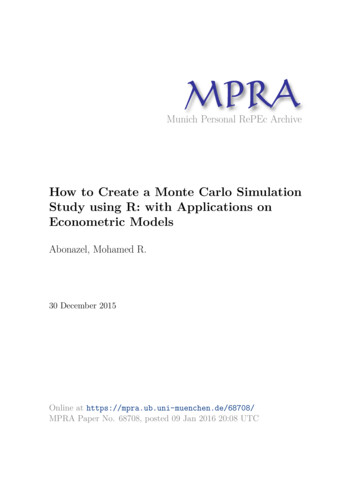
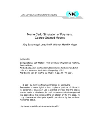
Example: Fertility There are 2.256 million 25-year-old women in the UnitedStates, and they have a 9.4 percent average probability ofhaving a child. For this example, assume a 1/1000 sample, so there are2,256 representative individuals (women) in the model. In a nonmicro model, the number of children born would bethe number of women in the group times the groupprobability. In a simple microsimulation, a random number is drawn foreach individual, and a child is assigned to that individual if therandom number is lower than the individual’s probability ofhaving a child.CONGRESSIONAL BUDGET OFFICE5
Distribution of Number of Children After 1,000 Runs of aSimple MicrosimulationNumber of r of Children230240250 In a nonmicro model: 2,256 women 9.4 percent 212 childrenCONGRESSIONAL BUDGET OFFICE6
Small Changes Matter in a Dynamic Microsimulation In a dynamic model, outcomes each year are based on themodel’s outcomes for the prior year. Changes propagate in later years in many ways.– Larger birth cohorts go on to have more children (on average).– Larger birth cohorts mean more workers, greater economic output,and eventually more Social Security spending.– Labor supply differs for mothers with children at home, which leadsto different hours, earnings, and output.– Probabilities are a function of the state of the model, so differentearnings, wages, etc. mean that individuals’ outcomes will changeeven when the same random numbers are used.CONGRESSIONAL BUDGET OFFICE7
Monte Carlo Variation Can Lead to Problems Any single run could be an outlier. Any change in the model can cause a propagating change.– Policy– Assumptions– Bug fixes Changes are unpredictable. However, those changes are limited to the size of the MonteCarlo variation—so even if we use the same random numbersin each model run, we still need to understand Monte Carlovariation.CONGRESSIONAL BUDGET OFFICE8
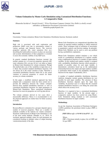
How Large Is the Monte Carlo Variation (and the Error)? Cannot be computed mathematically Determined empirically by Monte Carlo simulation usingvarying random numbers Different for different outcomes Generally small in comparison with the outcomes, but oftennot small in comparison with a proposed policy changeCONGRESSIONAL BUDGET OFFICE9
Distribution of OASDI 75-Year Actuarial ShortfallsAfter 100 Runs of a MicrosimulationNumber of ge of Taxable PayrollCONGRESSIONAL BUDGET OFFICE4.454.5010
Distribution of OASDI Outlays as a Percentage of GDPAfter 100 Runs of a MicrosimulationHighest95th Percentile75th PercentileAverage25th Percentile5th PercentileLowestOASDI Outlays as a Percentage of AL BUDGET OFFICE2080209011
Distribution of OASDI Outlays as a Percentage of GDPAfter 100 Runs of a Microsimulation: A Closer LookHighest95th Percentile75th PercentileAverage25th Percentile5th PercentileLowestOASDI Outlays as a Percentage of 40205020602070CONGRESSIONAL BUDGET OFFICE2080209012
Distribution of Differences From the Average in OASDI Outlaysas a Percentage of GDP After 100 Runs of a MicrosimulationPercentage Difference From Average of 100 Runs5432Highest195th Percentile75th Percentile025th Percentile5th NGRESSIONAL BUDGET OFFICE2080209013
Effect on OASDI Outlays as a Percentage of GDP From aChange of One Death in 2015, Single RunPercent7Base CaseChange of One Death654321Percentage 0 Perturb the model a tiny amount—in this case, by just a single deathin 2015 out of more than 2700 representative deaths—and changespropagate in later years.CONGRESSIONAL BUDGET OFFICE14
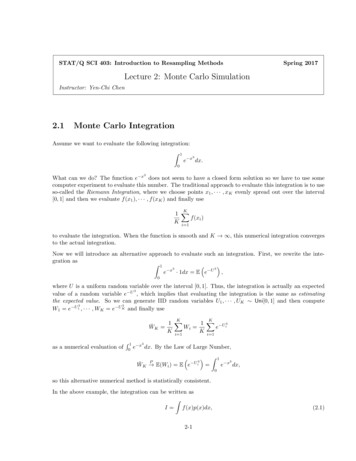
Effect on OASDI Outlays as a Percentage of GDP From aChange of One Death in 2015PercentBase Case(Single run)Change of One Death(Single run)76543Percentage Difference95th Percentileof the Monte CarloDistribution (100 runs)21Single Run05th Percentileof the Monte CarloDistribution (100 runs)-1-2201020202030204020502060207020802090 The changes are the same size as the Monte Carlo variation.CONGRESSIONAL BUDGET OFFICE15
Effect on OASDI Outlays as a Percentage of GDP From aTiny Change in the Benefit FormulaPercentBase Case(Single run)0.1 Percent Cut inInitial Benefits(Single run)76543Percentage Difference95th Percentileof the Monte CarloDistribution (100 runs)210Single Run5th Percentileof the Monte CarloDistribution (100 runs)-1-2201020202030204020502060207020802090 A tiny change in the benefit formula—in this case, a 0.1 percentcut in initial benefits—has similar effects in later years, againlimited to the size of the Monte Carlo variation.CONGRESSIONAL BUDGET OFFICE16
What Can Be Done? What Have We Done? Increase sample size Use targets from macro models to guide the microsimulation Pick a baseline run that has important values close to thecenter of the Monte Carlo distribution Average among many simulations that use different randomnumbersCONGRESSIONAL BUDGET OFFICE17
Increase Sample Size Increases memory requirements and computational time The additional data necessary may not be availableCONGRESSIONAL BUDGET OFFICE18
Use Targets From Macro Models to Guide theMicrosimulation Uses random numbers combined with modeled probabilities torank individuals; then selects the highest-ranked individuals untila macro-derived target is reached Typically used to keep the simulation on track over longerperiods of time Does not eliminate Monte Carlo variation! Becausecharacteristics vary among the individuals in the model, therandom numbers still matter to outcomes Used in CBOLT for various processes, such as the mortalityprocess example shown earlierCONGRESSIONAL BUDGET OFFICE19
Pick a Baseline Run That Has Important ValuesClose to the Center of the Monte Carlo Distribution Easy to do if the model is built to select one of the MonteCarlo runs Avoids a very likely move back toward the center ofdistribution with perturbation of the model if the baseline runwere to be an outlierCONGRESSIONAL BUDGET OFFICE20
Distribution of OASDI 75-Year Actuarial ShortfallsAfter 100 Runs of a MicrosimulationNumber of SimulationsSelected Single-Run Baseline141210864204.204.254.304.354.40Percentage of Taxable PayrollCONGRESSIONAL BUDGET OFFICE4.454.5021
Average Among Many Simulations That Use DifferentRandom Numbers May be used when more precision is needed Effective in reducing error No increased memory or additional data needed Increases computing time Need to determine reasonable number of runs, which is atrade-off between error and the time that the modeling takesCONGRESSIONAL BUDGET OFFICE22
Effect on OASDI Outlays as a Percentage of GDP From aChange of One Death in 2015Percent7Base Case(Single run)6Change of One Death(Single run)543Percentage Difference95th Percentileof the Monte CarloDistribution (100 runs)Single Run2105th Percentileof the Monte CarloDistribution (100 runs)-1-2201020202030204020502060207020802090 Change one death in 2015, and costs can differ by /- 1 percent.CONGRESSIONAL BUDGET OFFICE23
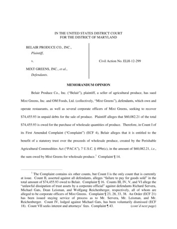
Effect on OASDI Outlays as a Percentage of GDP From aChange of One Death in 2015, Averaging Among RunsPercent7Base Case(Average of 30 runs)6Change of One Death(Average of 30 runs)543Percentage Difference95th Percentileof the Monte CarloDistribution (100 runs)210Average of 30 Runs5th Percentileof the Monte CarloDistribution (100 runs)-1-2201020202030204020502060207020802090 Change one death in 2015, but do 30 Monte Carlo runs;variation is reduced greatly.CONGRESSIONAL BUDGET OFFICE24
Effect on OASDI Outlays as a Percentage of GDP From aCut in Benefits, Comparing a Single Run to AveragingPercent7Base Case(Single run)60.1 Percent Cut inInitial Benefits(Single run)543Percentage Difference95th Percentileof the Monte CarloDistribution (100 runs)Average of 30 RunsSingle Run5th Percentileof the Monte CarloDistribution (100 runs)210-1-2201020202030204020502060207020802090 The effect is the same with the tiny cut in benefits.CONGRESSIONAL BUDGET OFFICE25
Example: A 5 Percent Cut in Initial OASDI Benefits,Single Run The path of changes has a lot of noise even after the effect ofthe policy is fully phased in. When the effect is fully phased in, annual changes could be3.5 percent to 6 percent, depending on the year.CONGRESSIONAL BUDGET OFFICE26
Effect on OASDI Outlays as a Percentage of GDP From a5 Percent Cut in Initial Benefits in 2015, Single RunPercent8Base Case5 Percent Cut inInitial Benefits6420-2-4Percentage IONAL BUDGET OFFICE2080209027
Example: A 5 Percent Cut in Initial OASDI Benefits,Average of 30 Runs The paths of outlays as a percentage of GDP are smoother, andthe path of changes is much smoother, varying only from about4.7 percent to 4.9 percent once the effect is fully phased in. Noise is a function of the number of runs; more could be used.CONGRESSIONAL BUDGET OFFICE28
Effect on OASDI Outlays as a Percentage of GDP From a5 Percent Cut in Initial Benefits in 2015, Average of 30 RunsPercent8Base Case5 Percent Cut inInitial Benefits6420-2-4Percentage IONAL BUDGET OFFICE2080209029
Example: A 5 Percent Cut in Initial OASDI Benefits,Effects on the Actuarial Shortfall Center of distributions improves the shortfall by 0.7 percentagepoints of taxable payroll (16 percent) Estimate of improvement could be skewed if single runs areused and outcomes are outliers– “Outside” outliers would show an improvement of 0.9 percentagepoints (20 percent)– “Inside” outliers would show an improvement of 0.4 percentage points(10 percent)CONGRESSIONAL BUDGET OFFICE30
Distribution of OASDI 75-Year Actuarial Shortfalls in theBase Case and With a 5 Percent Cut in Initial BenefitsFrequency0.25With a 5 PercentCut in Initial Benefits(30 Runs)0.20Base Case(100 ntage of Taxable PayrollCONGRESSIONAL BUDGET OFFICE4.34.44.531
Conclusion Monte Carlo variation exists in all microsimulations. Minute changes to policy or the model create propagatingchanges; these changes are essentially Monte Carlo variation. Both triggers of variation can cloud outcomes. Techniques exist to minimize the negative effects. Knowing the distribution of Monte Carlo variation foroutcomes of interest helps determine the appropriatetechnique.CONGRESSIONAL BUDGET OFFICE32
Determined empirically by Monte Carlo simulation using varying random numbers Different for different outcomes Generally small in comparison with the outcomes, but often . The changes are the same size as the Monte Carlo variation. Percent Base Case (Single run) Change of One Death (Single run) 5th Percentile of the Monte Carlo Distribution .