WIXLIB

STAT/Q SCI 403: Introduction to Resampling MethodsSpring 2017Lecture 2: Monte Carlo SimulationInstructor: Yen-Chi Chen2.1Monte Carlo IntegrationAssume we want to evaluate the following integration:Z13e x dx.03What can we do? The function e x does not seem to have a closed form solution so we have to use somecomputer experiment to evaluate this number. The traditional approach to evaluate this integration is to useso-called the Riemann Integration, where we choose points x1 , · · · , xK evenly spread out over the interval[0, 1] and then we evaluate f (x1 ), · · · , f (xK ) and finally useK1 Xf (xi )K i 1to evaluate the integration. When the function is smooth and K , this numerical integration convergesto the actual integration.Now we will introduce an alternative approach to evaluate such an integration. First, we rewrite the integration asZ 1 33e x · 1dx E e U ,0where U is a uniform random variable over the interval [0, 1]. Thus, the integration is actually an expected3value of a random variable e U , which implies that evaluating the integration is the same as estimatingthe expected value. So we can generate IID random variables U1 , · · · , UK Uni[0, 1] and then compute33W1 e U1 , · · · , WK e UK and finally useW̄K as a numerical evaluation ofR10KK1 X Ui31 XWi eK i 1K i 13e x dx. By the Law of Large Number, Z3PW̄K E(Wi ) E e Ui 13e x dx,0so this alternative numerical method is statistically consistent.In the above example, the integration can be written asZI f (x)p(x)dx,2-1(2.1)

2-2Lecture 2: Monte Carlo Simulationwhere f is some function and p is a probability density function. Let X be a random variable with densityp. Then equation (2.1) equalsZf (x)p(x)dx E(f (X)) I.Namely, the result of this integration is the same as the expected value of the random variable f (X). Thealternative numerical method to evaluate the above integration is to generate IID X1 , · · · , XN p, N datapoints, and then use the sample averageN1 XIbN f (Xi ).N i 1This method, the method of evaluating the integration via simulating random points, is called the integrationby Monte Carlo Simulation.An appealing feature of the Monte Carlo Simulation is that the statistical theory is rooted in the theory ofsample average. We are using the sample average as an estimator of the expected value. We have alreadyseen that the bias and variance of an estimator are key quantities of evaluating the quality of an estimator.What will be the bias and variance of our Monte Carlo Simulation estimator?The bias is simple–we are using the sample average as an estimator of it expected value, so the bias(IbN ) 0.The variance will then be1Var(IbN ) Var(f (X1 ))N 1 22 E(f (X1 )) E (f (X1 )) {z }N(2.2)I2 Z 1 f 2 (x)p(x)dx I 2 .NRThus, the variance contains two components: f 2 (x)p(x)dx and I 2 .Given a problem of evaluating an integration, the quantity I is fixed. What we can choose is the number ofrandom points N and the sampling distribution p! An important fact is that when we change the samplingdistribution p, the function f will also change.R13For instance, in the example of evaluating 0 e x dx, we have seen an example of using uniform random variables to evaluate it. We can also generate IID B1 , · · · , BK Beta(2, 2), K points from the beta distributionBeta(2,2). Note that the PDF of Beta(2,2) ispBeta(2,2) (x) 6x(1 x).We can then rewriteZ1e0 x3Zdx 013e x· 6x(1 x) dx E6x(1 x) {z } {z }p(x)3e B16B1 (1 B1 )!.f (x)What is the effect of using different sampling distribution p? The expectation is alwaysR fixed to be I so thesecond part of the variance remains the same. However, the first part of the variance f 2 (x)p(x)dx dependshow you choose p and the corresponding f .Thus, different choices of p leads to a different variance of the estimator. We will talk about how to choosean optimal p in Chapter 4 when we talk about theory of importance sampling.

Lecture 2: Monte Carlo Simulation2.22-3Estimating a Probability via SimulationHere is an example of evaluating the power of a Z-test. Let X1 , · · · , X16 be a size 16 random sample. Letthe null hypothesis and the alternative hypothesis beH0 : Xi N (0, 1),Ha : Xi N (µ, 1), where µ 6 0. Under the significance level α, the two-tailed Z-test is to reject H0 if 16 X̄16 z1 α/2 ,where zt F 1 (t), where F is the CDF of the standard normal distribution. Assume that the true valueof µ is µ 1. In this case, the null hypothesis is wrong and we should reject the null. However, due tothe randomness of sampling, we may not be able to reject the null every time. So a quantity we will beinterested in is: what is the probability of rejecting the null under such µ? In statistics, this probability (theprobability that we reject H0 ) is called the power of a test. Ideally, if H0 is incorrect, we want the power tobe as large as possible.What will the power be when µ 1? Here is the analytical derivation of the power (generally denoted asβ):β P (Reject H0 µ 1) X̄16 N (µ, 1/16) P ( 16 X̄16 z1 α/2 µ 1), P (4 · N (1, 1/16) z1 α/2 )(2.3) P ( N (4, 1) z1 α/2 ) P (N (4, 1) z1 α/2 ) P (N (4, 1) z1 α/2 ) P (N (0, 1) z1 α/2 4) P (N (0, 1) 4 z1 α/2 ).Well.this number does not seem to be an easy one.What should we do in practice to compute the power? Here is an alternative approach of computing thepower using the Monte Carlo Simulation. The idea is that we generate N samples, each consists of 16 IIDrandom variables from N (1, 1) (the distribution under the alternative). For each sample, we compute theZ-test statistic, 16 X̄16 , and check if we can reject H0 or not (i.e., checking if this number is greater thanor equal to z1 α/2 ). At the end, we use the ratio of total number of H0 being rejected as an estimate of thepower β. Here is a diagram describing how the steps are carried out: RejectHgeneratescompute0 D1 Yes(1)/No(0)N (1, 1) 16 observations test statistic16 X̄16 RejectHgeneratescompute0N (1, 1) 16 observations test statistic16 X̄16 D2 Yes(1)/No(0).generatescomputeN (1, 1) 16 observations test statistic RejectH016 X̄16 DN Yes(1)/No(0)Each sample will end up with a number Di such that Di 1 if we reject H0 and Di 0 if we do not rejectH0 .Because the Monte Carlo Simulation approach is to use the ratio of total number of H0 being rejected toestimate β, this ratio isPNj 1 DjD̄N .NIs the Monte Carlo Simulation approach a good approach to estimate β? The answer is–yes it is a goodapproach of estimating β and moreover, we have already learned the statistical theory of such a procedure!

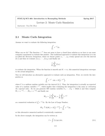
2-4Lecture 2: Monte Carlo SimulationThe estimator D̄N is just a sample average and each Dj turns out to be a Bernoulli random variable withparameterp P (Reject H0 µ 1) βby equation (2.3). Therefore, bias D̄N E(D̄N ) β p β 0 p(1 p)β(1 β)Var D̄N NN β(1 β)MSE D̄N , β .NThus, the Monte Carlo Simulation method yields a consistent estimator of the power:PD̄N β.Although here we study the Monte Carlo Simulation estimator of such a special case, this idea can be easilyto generalize to many other situation as long as we want to evaluate certain numbers. In modern statisticalanalysis, most papers with simulation results will use some Monte Carlo Simulations to show the numericalresults of the proposed methods in the paper.The following two figures present the power β as a function of the value of µ (blue curve) with α 0.10.The red curves are the estimated power by Monte Carlo simulations using N 25 and 100.0.80.6Power0.00.20.40.60.40.00.2Power0.81.0N 1001.0N 25 2 10µ12 2 10µ12 The gray line corresponds to the value of power being 0.10. Think about why the power curve (bluecurve) hits the gray line at µ 0.2.3Estimating Distribution via SimulationMonte Carlo Simulation can also be applied to estimate an unknown distribution as long as we can generatedata from such a distribution. In Bayesian analysis, people are often interested in the so-called posteriordistribution. Very often, we known how to generate points from a posterior distribution but we cannotwrite down its closed form. In this situation, what we can do is to simulate many points and estimate thedistribution using these simulated points. So the task becomes:

Lecture 2: Monte Carlo Simulation2-5given X1 , · · · , Xn F (or PDF p), we want to estimate F (or the PDF p).Estimating the CDF using EDF. To estimate the CDF, a simple but powerful approach is to use theEDF:n1XFbn (x) I(Xi x).n i 1We have already learned a lot about EDF in the previous chapter.Estimating the PDF using histogram. If the goal is to estimate the PDF, then this problem is calleddensity estimation, which is a central topic in statistical research. Here we will focus on the perhaps simplestapproach: histogram. Note that we will have a more in-depth discussion about other approaches in Chapter8.For simplicity, we assume that Xi [0, 1] so p(x) is non-zero only within [0, 1]. We also assume that p(x) issmooth and p0 (x) L for all x (i.e. the derivative is bounded). The histogram is to partition the set [0, 1](this region, the region with non-zero density, is called the support of a density function) into several binsand using the count of the bin as a density estimate. When we have M bins, this yields a partition: 11 2M 2 M 1M 1B1 0,, B2 ,, · · · , BM 1 ,, BM ,1 .MM MMMMIn such case, then for a given point x B , the density estimator from the histogram will bennumber of observations within B 1MXpbn (x) I(Xi B ).nlength of the binn i 1The intuition of this density estimator is that the histogram assign equal density valuePnto every points withinthe bin. So for B that contains x, the ratio of observations within this bin is n1 i 1 I(Xi B ), whichshould be equal to the density estimate times the length of the bin.Now we study the bias of the histogram density estimator.E (bpn (x)) M · P (Xi B )Z M Mp(u)du 1 M 1 M F FMM F M F 1M 1/M F M F 1M 1M M 1 p(x ), x ,.M MThe last equality is done by the mean value theorem with F 0 (x) p(x). By the mean value theorem again,there exists another point x between x and x such thatp(x ) p(x) p0 (x ).x x

2-6Lecture 2: Monte Carlo SimulationThus, the biasbias(bpn (x)) E (bpn (x)) p(x) p(x ) p(x) p0 (x ) · (x x)(2.4) p0 (x ) · x x L .MNote that in the last inequality we use the fact that both x and x are within B , whose total length is 1/M ,so the x x 1/M . The analysis of the bias tells us that the more bins we are using, the less bias thehistogram has. This makes sense because when we have many bins, we have a higher resolution so we canapproximate the fine density structure better.Now we turn to the analysis of variance.!n1XI(Xi B )n i 1Var(bpn (x)) M 2 · Var M2 ·P (Xi B )(1 P (Xi B )).nBy the derivation in the bias, we know that P (Xi B ) 2Var(bpn (x)) M ·p(x )Mp(x )M ,so the variance ) 1 p(xMnp(x ) p2 (x ) M· .nn(2.5)The analysis of the variance has an interesting result: the more bins we are using, the higher variance weare suffering.Now if we consider the MSE, the pattern will be more inspiring. The MSE isMSE(bpn (x)) bias2 (bpn (x)) Var(bpn (x)) p(x ) p2 (x )L2 M· .M2nn(2.6)An interesting feature of the histogram is that: we can choose M , the number of bins. When M is too large,the first quantity (bias) will be small while the second quantity (variance) will be large; this case is calledundersmoothing. When M is too small, the first quantity (bias) is large but the second quantity (variance)is small; this case is called oversmoothing.To balance the bias and variance, we choose M that minimizes the MSE, which leads to Mopt n · L2p(x ) 1/3.(2.7)Although in practice the quantity L and p(x ) are unknown so we cannot chose the optimal Mopt , the rule inequation (2.7) tells us how we should change the number of bins when we have more and more sample size.Practical rule of selecting M is related to the problem of bandwidth selection, a research topic in statistics.

by Monte Carlo Simulation. An appealing feature of the Monte Carlo Simulation is that the statistical theory is rooted in the theory of sample average. We are using the sample average as an estimator of the expected value. We have already seen that the bias and variance of an estimator are key quantities of evaluating the quality of an estimator.