Transcription
John von Neumann Institute for ComputingMonte Carlo Simulation of Polymers:Coarse-Grained ModelsJörg Baschnagel, Joachim P. Wittmer, Hendrik Meyerpublished inComputational Soft Matter: From Synthetic Polymers to Proteins,Lecture Notes,Norbert Attig, Kurt Binder, Helmut Grubmüller, Kurt Kremer (Eds.),John von Neumann Institute for Computing, Jülich,NIC Series, Vol. 23, ISBN 3-00-012641-4, pp. 83-140, 2004.c 2004 by John von Neumann Institute for ComputingPermission to make digital or hard copies of portions of this workfor personal or classroom use is granted provided that the copiesare not made or distributed for profit or commercial advantage andthat copies bear this notice and the full citation on the first page. Tocopy otherwise requires prior specific permission by the publishermentioned above.http://www.fz-juelich.de/nic-series/volume23
Monte Carlo Simulation of Polymers:Coarse-Grained ModelsJ. Baschnagel, J. P. Wittmer, and H. MeyerInstitut Charles Sadron,6, rue Boussingault, 67083 Strasbourg Cedex, FranceE-mail: {baschnag, jwittmer, hmeyer}@ics.u-strasbg.frA coarse-grained simulation model eliminates microscopic degrees of freedom and representsa polymer by a simplified structure. A priori, two classes of coarse-grained models may bedistinguished: those which are designed for a specific polymer and reflect the underlying atomistic details to some extent, and those which retain only the most basic features of a polymerchain (chain connectivity, short-range excluded-volume interactions, etc.). In this article wemainly focus on the second class of generic polymer models, while the first class of specificcoarse-grained models is only touched upon briefly. Generic models are suited to explore general and universal properties of polymer systems, which occur particularly in the limit of longchains. The simulation of long chains represents a challenging problem due to the large relaxation times involved. We present some of the Monte Carlo approaches contrived to cope withthis problem. More specifically, our review contains two main parts. One part (Sec. 5) dealswith local and non-local updates of a polymer. While local moves allow to extract informationon the physical polymer dynamics from Monte Carlo simulations, the chief aim of non-localmoves is to accelerate the relaxation of the polymers. We discuss some examples for suchnon-local moves: the slithering-snake algorithm, the pivot algorithm, and its recently suggestedvariant, the double-pivot algorithm, which is particularly suited for the simulations of concentrated polymer solutions or melts. The second part (Sec. 6) focuses on modern Monte Carlomethods that were inspired by the Rosenbluth-Rosenbluth algorithm proposed in the 1950s tosimulate self-avoiding walks. The modern variants discussed comprise the configuration-biasMonte Carlo method, its recent extension, the recoil-growth algorithm, and the pruned-enrichedRosenbluth method, an algorithm particularly adapted to the simulation of attractively interacting polymers.1IntroductionPolymers are macromolecules in which N monomeric repeat units are connected to formlong chains.a Experimentally the chain length N is large, typically 10 3 . N . 105 .The size of a chain ( 103 Å) thus exceeds that of a monomer ( 1Å) by several orders ofmagnitude. However, contrary to granular materials, 2 the chain is not so large that thermalenergyb would be unimportant. Not at all! Thermal energy is the important energy scalefor polymers. It provokes conformational transitions so that the polymer can assume amultitude of different configurations at ambient conditions. ca More precisely, this definition refers to “linear homopolymers”, i.e., linear chain molecules consisting of onemonomer species only. By contrast, polymer chemistry can nowadays synthesize various other topologies, suchas cyclic, star- or H-polymers. For a very commendable review on the physical chemistry of polymers see Ref. 1.b Here, we mean the thermal energy supplied at ambient temperature, i.e., k T 4.1 · 10 21 J for T 300 K.Bc Polymers are a paradigm for “soft matter” materials or “complex fluids”. Roughly speaking, “soft matter”consists of materials whose constituents have a mesoscopic size (microscopic scale 1 Å mesoscopic object 102 104 Å macroscopic scale 1mm) and for which kB T is the important energy scale (whence thesoftness at ambient conditions). Examples other than polymers are colloidal suspensions, liquid crystals, or fluidmembranes.383
Changes of the configurations occur on very different scales, ranging from the localscale of a bond to the global scale of the chain. 4, 5 This separation of length scales entailssimplifications and difficulties. Simplifications arise on large scales where the chain exhibits universal behavior. That is, properties which are independent of chemical details. 6, 7These properties may be studied by simplified, “coarse-grained” models, e.g. via computer simulations. For simulations the large-scale properties, however, also give rise to aprincipal difficulty. Long relaxation times are associated with large chain lengths. 7–9The present chapter focuses on some of the Monte Carlo approaches to cope with thisdifficulty. Why Monte Carlo? Within a computational framework it appears natural toaddress dynamical problems via the techniques of Molecular Dynamics (see Ref. 10). AMolecular Dynamics (MD) simulation numerically integrates the equations of motion ofthe (polymer) system, and thereby replicates, authentically, its (classical) dynamics. As thepolymer dynamics ranges from the (fast) local motion of the monomers to (slow) largescale rearrangements of a chain, there is a large spread in time scales. The authenticityof MD thus carries a price: Efficient equilibration and sampling of equilibrium propertiesbecomes very tedious –sometimes even impossible– for long chains. At that point, MonteCarlo simulations may provide an alternative. Monte Carlo moves are not bound to belocal. They can be tailored to alter large portions of a chain, thereby promising efficientequilibration. The discussion of such moves is one of the gists of this review.Outline and Prerequisites. The plan of the chapter is as follows: We begin by gatheringnecessary background information, both as to polymer physics (Sec. 2) and as to the MonteCarlo method (Sec. 3). Then, we present the simulation models (Sec. 4), which have beenused to develop and to study various Monte Carlo algorithms. The discussion of these algorithms (Secs. 5 and 6) represents the core of the chapter. Section 5 deals with local moves,allowing to study the physical polymer dynamics via Monte Carlo, and non-local moves(slithering-snake algorithm, pivot algorithm, double-pivot algorithm), aiming at speedingup the relaxation of the chains. Section 5 discusses the Rosenbluth-Rosenbluth method forsimulating self-avoiding walks and some of its modern variants (pruned-enriched Rosenbluth method, configuration-bias Monte Carlo, recoil-growth algorithm). The last section(Sec. 7) briefly recapitulates the different methods and gives some advice when to employ which algorithm. Finally, the appendix 7 reviews a recently proposed approach tosystematically derive coarse-grained models for specific polymers.Our presentation is based on the following prerequisites: We will restrict our attention to homopolymers, i.e., to polymers consisting of onemonomer species only. However, (some of) the algorithms discussed may also beapplied e.g. to polymer blends or block-copolymers (see Ref. 11). The chains are monodisperse, i.e, N is constant. We do not consider long-range (e.g., electrostatic) or specific (e.g., H-bonds) interactions between the monomers. These interactions are treated in other chapters (e.g.,see Refs. 12, 13). We do not treat the solvent molecules explicitly. They are indirectly accounted forby the interactions between the monomers. The neglect of the solvent does not affect84
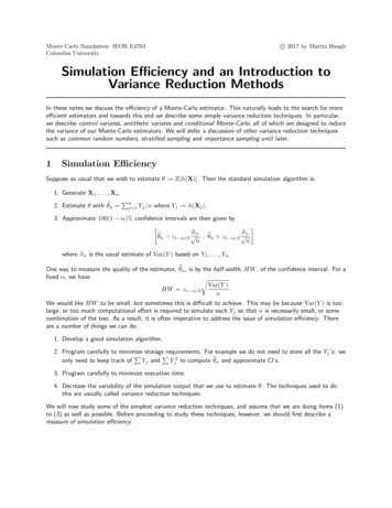
the static properties of chains in dilute solution. However, it does affect their physicaldynamics (see Ref. 14).2A Primer to Polymer Physics2.1 A Polymer in Good SolventTo substantiate the remarks of the introduction about the large-scale properties of polymerslet us consider a specific example, a dilute solution of polyethylene. Polyethylene consistsof CH2 -monomers which are joined to form a linear polymer (Fig. 1). A configuration ofthe chain may be specified by the positions of the monomers d x (r 1 , . . . , r N ). Thermodynamic properties are calculated by averaging an observable A over all configurationsZ 1hAi dx A(x) exp βU (x) .(1)ZHere β kB T , Z is the partition function and U (x) the interaction potential. We assumethat U (x) can be split into two parts:eU (x) N 1Xi 1U0 (bi , . . . , bj , . . . , bi imax ) U1 (x, solvent) ,{z}{z} “short-range”: ,θ,φ,.(2)“long-range”where bi r i 1 r i denotes the bond vector from the ith to the (i 1)th monomer.The first term of Eq. (2), U0 , depends on the chemical nature of the polymer. It comprises the potentials of the bond length , the bond angle θ, the torsional angle φ, etc.(Fig. 1).17 These potentials lead to correlations between the bond vectors b i and bj . Typically, the correlations are of short range: they only extend up to some bond vector b j i imaxwith imax N .Although distant monomers along the backbone of the chain are thus orientationallydecorrelated, they can still come close in space. The resulting interaction is long-rangealong the chain backbone (Fig. 1). In Eq. (2), it is accounted for by the second termU1 .6, 7 U1 depends strongly on the quality of the solvent. f In good solvents the monomerseffectively repel one another (they want to be surrounded by solvent molecules), whereasthey attract each other if the solvent cannot dissolve the polymer (bad solvent).Due to its long-range character, one intuitively expects U 1 to influence the large-scalebehavior of the chain more strongly than U0 . A possible test of this idea is to estimate howthe size of a chain scales with N . Common measures of the chain size are the mean-squareend-to-end distance Re2 or the radius of gyration Rg2 (Fig. 1)DERe2 (r N r 1 )2 ,Rg2 N 2 E1 XDr i Rcm,N i 1(3)d Here, we adopt a description in terms of a so-called “united atom model”. The united atom model represents a CH2 -group by a single, spherical interaction site and does not distinguish between inner (CH 2 ) and endmonomers (CH3 ).15 Furthermore, we neglect the momenta of the monomers to specify the configuration, as weassume the observables and interaction potentials to depend on positions only.e Equation (1) does not contain the degrees of freedom of the solvent. They are assumed to be integrated out.Thus, U (x) is an effective potential –in fact, a free energy– depending on the properties of the solvent.f In Eq. (2) we assume that U is independent of the solvent quality.085
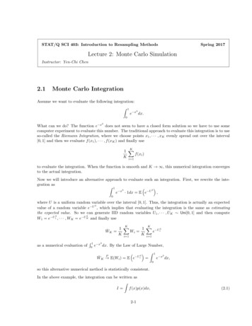
persistence length p 5Åradius of gyration RgCH2φ CH2H2CH2CCH2CH2θ HC2cmCH2end-to-end distanceN 104 : Re 103 Åvbond length 0 1Åglobal properties universal:polymer critical system1/N (T Tc )/Tc τlocal propertiesdepend on chemistryRe Rg N ν ξ τ νFigure 1. Schematic illustration of polyethylene. The local properties of the polymer depend on its microscopicdegrees of freedom: the bond length , the bond angle θ, and the torsional angle φ. Because the potential ofthe bond length is fairly “stiff”, may be kept fixed at its equilibrium value 0 in a modeling approach. Bycontrast, the potential of the torsional angle is much “softer”. Thus, φ, which characterizes rotations abouta middle C-C bond, mainly determines the local conformation of the chain. All degrees of freedom ( , θ, φ)determine the intrinsic stiffness of the chain. The stiffness reflects the persistence of orientational correlationsalong the backbone of the chain. Orientational correlations decouple on the length scale of the “persistencelength” p . For typical chain lengths, N 104 , p is much smaller than the end-to-end distance Re or theradius of gyration Rg . (Rg measures the average distance of a monomer from the center of mass (cm) of thechain.) Thus, the chain appears flexible on length scales larger than p . If the polymer is dissolved in a goodsolvent, distant monomers (filled grey circles) repel each other when they come in contact. That is, the excludedvolume parameter v, measuring the effective interaction between distant monomers along the chain, is positive.Under these conditions (i.e., linear polymer with some flexibility and repulsive monomer-monomer interactions) acorrespondence between the large-scale properties of the polymer and a critical system close to its phase transitioncan be established:6, 16 1/N may be identified with the reduced distance, τ , to the critical temperature T c of thephase transition, and Re or Rg scale with N as the correlation length ξ of the order parameter does with τ . ν isa universal critical exponent, often called “Flory exponent” in polymer science.where Rcm is the position of the chain’s center of mass. Because R e Rg we focus on Rein the sequel to illustrate the role played by U 0 and U1 .Let b̂i denote the unit vector associated with the bond b i of fixed length 0 (Fig. 1).Then, quite generally, we may write Re2 asRe2 20 1N 1 NXXi 1 j 1hb̂i · b̂j i 2 20 1 iN 1 NXXi 1k 0hb̂i · b̂i k i (N 1) 20 .(4)Apparently, the large-scale behavior of Re depends on the range of orientational correlations between bond vectors. Two cases may be distinguished: gg Inpart, the subsequent discussion closely follows that on p. 148 of Ref. 18.86
1. If hb̂i · b̂i k i is “short-range”, i.e., if it decays more rapidly than 1/k for large k, thesecond term converges in the large-N limit. Then, X phb̂1 · b̂1 k i 1 : N 20 2 1Re2 N 20 2(N ) ,(5) 0k 0where we introduce the persistence length p in the last term. ( p measures the “persistence” of orientational correlations along the backbone and thus the intrinsic stiffnessof the chain; see Fig. 1). Equation (5) shows that short-range orientational correlationsonly affect the prefactor –they renormalize the bond length to b 0 [2( p / 0 ) 1]1/2(b is called “effective bond length”7 )– but they do not change the scaling of Re withN . The scaling is always “random-walk-like”: h Re N 1/2 .7 In polymer science, achain exhibiting this random-walk-like behavior is commonly referred to as an “idealchain”.Of course, the finite-range correlations, assumed for U 0 in Eq. (2), are also of shortrange. Thus, provided U1 0, the end-to-end distance of a (long) chain is givenby Re bN 1/2 , irrespective of the precise form of U0 . The microscopic degreesof freedom, , θ, φ, determine the prefactor, the effective bond length b, but not thescaling with N . Therefore, if we are interested in studying large-scale properties, wecan replace a chemically realistic model for polyethylene by a much simpler “coarsegrained model”, which is microscopically unrealistic, but correctly reproduces thelarge-N behavior. An example for such a coarse-grained model is a “bead-springmodel”, where N effective monomers (“beads”) are connected by harmonic springsof average length b (Fig. 2).2. However, if hb̂i · b̂i k i decays as 1/k or more slowly (as 1/k y with y 1) due tolong-range correlations, the scaling behavior of R e2 is changed. Instead of Re2 Nwe find 2 yZ NN(y 1) ,22Re N 0dk hb̂(k) · b̂(0)i (6)N ln N (y 1) .Thus, long-range correlations lead to a “swelling” of the chain size with respect to apure random walk.Such long-range correlations are embodied in the potential U 1 in Eq. (2). For a polymer in a good solvent a swelling of the chain dimension is physically reasonable.As soon as two (distant) monomers come close in space, they repel each other. Onthe level of the coarse-grained bead-spring model we can incorporate this repulsiveinteraction by writing U1 as (see e.g. Ref. 7 or the lucid discussion on pp. 16–20 ofRef. 16)ZNX 1U1 (r N ) d3 r kB T vρ(r)2 with ρ(r) δ r ri .(7)2i 1h By the term “random-walk-like” we mean the diffusional motion of a Brownian particle. This motion can bethought of as resulting from the addition of many small displacements in random directions so that the overallmean-square displacement of the particle in time t, R 2 (t) h[r(t) r(0)]2 i, scales as R2 t. This allowsfor the following identifications in regard to polymer physics: R Re and t N .87
H2CbU0 b H2CNXi 1bCH2φCH2θ HC2U0 (bi , . . . , bi imax ) U0bs N 1N 1 23kB T X 23kB T Xr i r i 1b i222b i 12b i 1Figure 2. From a chemically realistic model to a coarse-grained bead-spring model. Local properties of therealistic model are determined by its microscopic degrees of freedom: , θ, and φ. On the global level of thechain, however, the influence of the microscopic degrees of freedom can be lumped into one parameter, theeffective bond length b. The microscopic degrees of freedom do not determine the scaling of the end-to-enddistance, which, under the sole effect of U0 , is given by Re bN 1/2 (“ideal chain”). This behavior maybe recovered from Eq. (1) when calculating Re with the potential U0bs of a coarse-grained bead-spring model.This model identifies the monomers with spherical “beads” which are bound to one another by harmonic springswith force constant 3kB T /b2 . (This bead-spring model is often called “Gaussian chain” model in the polymerliterature.7 )Here, ρ(r) is the monomer density at point r and v ( 0) is the excluded-volumeparameter. v measures the strength of the repulsion of a binary contact between twobeads. Because a binary contact occurs with probability ρ(r) 2 , Eq. (7) expresses thetotal energy penalty resulting from the repulsive contacts of all beads in the chain.From the previous discussion of U0 and U1 the following conclusion may be drawn: Whenfocusing on the large-scale properties of linear polymers with some flexibility and predominantly repulsive interactions we may forego a microscopic description in favor of acoarse-grained model. An example is the bead-spring model introduced above (Fig. 2),which is characterized by two parameters, b and v. Another possibility is a self-avoidingwalk (SAW) on a (hyper-cubic) lattice. That is, a random walk which is not allowed tovisit an already occupied lattice site again (see Sec. 4.1). The replacement “microscopicmodel SAW” is permissible because a linear polymer in good solvent can be shown tocorrespond to a critical system which undergoes a phase transition for N (Fig. 1). Itbelongs to the universality class of the n-vector model in the limit n 0. 6, 16 This impliesthat the large-N behavior is determined by critical exponents. For instance,Rg Re bN νor Z µN N γ 1(N ) ,(8)where the partition function Z counts the number of N -step SAW’s starting at the originand ending anywhere. The connectivity constant µ and the bond length b are non-universal.They depend on the polymer and the external conditions (temperature, solvent, etc.). Bycontrast, the critical exponents ν and γ are universal. They only depend on the dimensionof space.i Thus, they can be determined for all polymers by studying this (simple) model.i In the course of the research on critical phenomena it has become clear that all systems with short-range, isotropic88
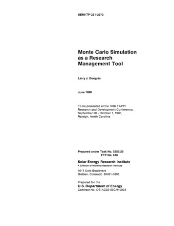
T 1/2Tθsemidilute (II)ν 1/2dilute (II)ν 1/2Tc(N)dilute (III)ν 1/3two phase regionρ (1)coexρc(N)ρ (2)coexglassy/semicrystalline meltN(liquid) meltsemidilute (I)ν 1/2dilute (I)ν 0.588ρFigure 3. Schematic phase diagram of flexible polymers (see Chap. 9 of Ref. 16 or Chap. 4 of Ref. 23). Forsmall monomer density ρ the solution is dilute. Three different regimes may be distinguished according to thetemperature T : swollen chains [Eq. (8), T TΘ : dilute (I)], nearly ideal chains [Eq. (10), T TΘ : dilute(II)], and collapsed chains [Eq. (11), T TΘ : dilute (III)]. There is an interval T around the Θ-point oforder T /TΘ 1/ N , where the chains are nearly ideal. Whereas the chains may be considered as beingisolated in dilute solution, they strongly overlap in the semidilute regimes. For T T c (N ) phase separation in adilute phase of collapsed chains and a semidilute solution of nearly ideal chains occurs. If the monomer densityapproaches 1, we obtain a polymer melt. At high T the melt is a (viscous) liquid, whereas at low T it may becomea glassy24 or a semicrystalline25 solid, depending on the ability of the polymer to form ordered structures or not.In fact, the currently most precise values of ν and γ (see footnote on page 112) have beenobtained from high-precision Monte Carlo simulations of SAW’s. 21, 222.2 Phase Diagram of a Polymer SolutionThe utility of coarse-grained models to investigate the statistical physics of polymer systems is not limited to the previous example. A dilute solution in a good solvent is justone region in the phase diagram. The phase diagram of flexible polymers is schematicallyshown in Fig. 3. Out of the various regimes we choose to discuss two cases in more detail,a chain in another than good solvent and (high-temperature) polymer melts. In the following sections we concentrate on those cases because novel Monte Carlo approaches havebeen applied to them.interactions, the same dimension of space d, and the same dimensionality n of the order parameter (n 1: scalar,n 2: n-dimensional vector) have critical exponents which depend only on (d, n) and take the same values asthose of the n-vector model.19, 2089
A Chain in a Θ-Solvent or a Bad Solvent. To extend the discussion of the good solventto other solvents let us reconsider Eq. (7). This equation corresponds to the first term of avirial expansion in the monomer density ρ(r). That is, 7, 16 Z11U1 d3 r kB T vρ(r)2 kB T wρ(r)3 . . . .(9)26This identifies the excluded-volume parameter v with the second virial coefficient. Ingeneral, the virial coefficients depend on temperature T . The second virial coefficientvanishes at some temperature, called “Θ-temperature T Θ ” in polymer science, and behavesas v v0 (1 TΘ /T ) close to the Θ-point (v0 const. 0). This implies that we cantune the solvent quality by temperature. In addition to the case of a good solvent (T T Θ )two further cases may be distinguished:1. Θ-solvent (T TΘ ): Since binary interactions are absent [but ternary interactions arepresent: w 0 in Eq. (9)], the polymer behaves nearly as an ideal chain: 16 (10)Re Rg N ( ln N corrections) .2. Bad solvent (T TΘ ): Since the binary interactions are attractive, the polymer iscollapsed to a dense sphere of monomers, implying that the average monomer densityρ inside the sphere is of order 1. Thus,N1ρ 3 1 Re Rg N ν with ν .(11)Rg3The simulation of this situation is complicated because the time to equilibrate thechain and to sample equilibrium properties from many independent configurationsbecomes exceedingly long. Two factors are responsible for that. On the one hand,the local dynamics is sluggish (maybe even glass-like) due to the dense packing ofmonomers that strongly attract each other. On the other hand, the polymer is entangledwith itself. Bonds cannot pass through each other. These topological constraints mayalso lead to slow dynamics for long chains.The Size of a Chain in a Polymer Melt. In a good solvent a chain expands with respect to theideal state, owing to long-range monomer-monomer repulsions. This is peculiar to dilutesolutions. In a dense liquid of chains, a “polymer melt”, the situation is quite different.One can show6, 7, 26 that the intra-chain excluded-volume interactions are screened by thepresence of the surrounding polymers. Thus, a chain in a melt behaves on large scales asan ideal chain, implying Re Rg N 1/2 (see Fig. 4).This ideality, first proposed by Flory,17 appears fairly unexpected. Some feeling whythis should be so may be obtained from the following argument: Inside the volume of achain ( Rg3 ) the monomer density resulting from the N monomers of the chain is verysmall. For ideal chains it is of order N/Rg3 N 1/2 , whereas it scales as N 0.764under good solvent conditions (using Eq. (8) and ν 0.588). We see that in dilute solution,swelling reduces the monomer density inside the chain and thus the total interaction energy[see Eq. (7)]. However, no energetic advantage may be gained in a melt because the overallmonomer density is ρ 1. Swelling would reduce the number of intra-chain contacts, butthis reduction must be compensated by inter-chain contacts to keep ρ constant. Thus, achain has to have N 1/2 contacts with other chains, which is huge in the large-N limit.This strong interpenetration of the chains suppresses the expansion of an individual chain.90
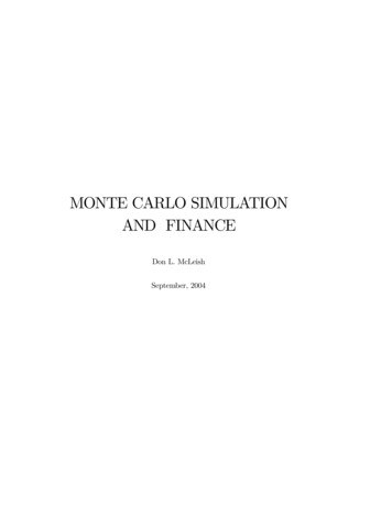
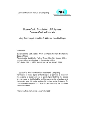
3102108.58φ 0 (dilute)φ 0.03125φ 0.5 (melt)inhaclenlwoSomndξ(φ 0.03125) 69.3.50ν er:alkWReRa 0:ν2 1/2〈(ri ri k) 〉 forN 32768,φ 0.03125110g(φ 0.03125) 209010010110210310N or k410Figure 4. End-to-end distance Re versus chain length N for the (athermal) bond-fluctuation model which willbe discussed in more detail in Secs. 4.1 and Sec. 5. Results for three volume fractions (of occupied lattice sites)are given, illustrating the dilute (φ 0), the semidilute (φ 0.03125) and the melt (φ 0.5) limits of theschematic phase diagram (Fig. 3). Using the slithering-snake algorithm (Sec. 5.2) it is possible to simulate chainscontaining up to N 32768 monomers for φ 0.5. Since the slithering-snake algorithm becomes less efficientat high densities (Sec. 5.2), the recently proposed double-pivot algorithm, described in Sec. 5.3, was harnessedto probe systems of higher densities (φ 0.5). Periodic boxes of linear size L 512 and containing up to222 monomers are required to eliminate finite-size effects. Such periodic boundary conditions are not neededfor single chains. Here, an infinite box was used (L(φ 0) ). As only excluded-volume interactionsare taken into account, good solvent statistics applies in dilute solution. The chains are swollen, as indicated bythe exponent ν 0.588 (solid line), which fits the data over three orders of magnitude. In the opposite (socalled) melt limit long-range correlations appear to be screened down to small chain lengths of about N 10(grey dashed line).27 Both chain statistics are visible for the intermediate density (φ 0.03125): Small chains(N g, Re ξ) are swollen (solid line) and long chains are Gaussian (dashed line). The intercept of bothlines defines the size ξ of the “excluded volume blob”6, 7 and the number of monomers g that the blob contains.The indicated numbers are specific to the volume fraction (and persistence length) given, but are independent ofchain length. For a given density ξ corresponds to the chain size where the coils start to overlap. Also presentedin the figure is the spatial distance h(r i r i k )2 i1/2 along the longest chain for φ 0.03125 (dotted line).With the exception of small N or k (i.e., N, k 10) this distance is, within the numerical accuracy of the data,identical to Re (N ) with N k. This agreement also demonstrates that the difference between a segment ofa long chain and a chain having the same length as the segment becomes irrelevant for distances larger than ξ.In precisely this sense the (long-range) excluded volume interactions are screened in semidilute solutions and inmelts. Mean-field descriptions become appropriate on the level of coarse-grained (Gaussian) chains of blobs. 6, 72.3 Dynamics of Polymer Melts: Rouse and Reptation ModelsThe Rouse Model. As a monomer in a dilute solution moves, it creates a vortex (“wave”) inthe solvent. The solvent transports the “wave” which is transported to other monomers ofthe chains so that a coupling between the motion of (distant) monomers arises (see Ref. 14).This long-range hydrodynamic interaction becomes screened by other chains when theconcentration of the solution increases.7 In a dense melt, hydrodynamic interactions arecompletely suppressed. Thus, it is generally believed that the Rouse theory 6, 7 providesa viable description for the long-time behavior of polymer dynamics in a melt, providedentanglements with other chains, giving rise to reptation dynamics, 7, 9 are not important91
neighbor chainsdTprimitive pathtube ˆchain topologyend-to-end distanceFigure 5. Sketch of the reptation concept for the dynamics of long-chain polymer melts. 7, 9 The chain is supposedto be enclosed in a “tube” formed by its neighbors. The tube may be characterized by an axis, the primitivepath. The tube confines the motion of the enclosed chain: It predominantly moves along the primitive path.Perpendicular excursions are suppressedbeyond the tube diameter dT . The tube diameter is larger than the effective bond length b: dT b Ne , where the “entanglement length” Ne 1. The primitive path representsthe shortest connection between the chain ends, which respects the topology imposed on the enclosed chain by theentanglements with its neighbors. The length L of the primitive path is thus larger than R e , which is the shortestconnection between the chain ends in space. L varies linearly with N : Ld T Re2 so that L dT (N/Ne ).(see Fig. 5 and also below).jThe Rouse theory assumes the chains to be ideal and models them as a sequence ofBrownian beads, connected by harmonic springs and subjected to a local random forceand a local friction.6, 7 This bead-spring model is characterized by two parameters: theeffective bond length b and the monomer mobility m. The mobility, or more precisly1/m, measures the time it takes a bead to diffuse over the distance b. Thus, the diffusioncoefficient of a monomer is proportional to mb 2 . As the center of mass (CM) of a chaindoes not experience any external force other than the antagonistic friction and randomforces, the theory predicts that the CM diffuses freely at all timesD 2 Eg3 (t) Rcm (t
Carlo method (Sec. 3). Then, we present the simulation models (Sec. 4), which have been used to develop and to study various Monte Carlo algorithms. The discussion of these algo-rithms (Secs. 5 and 6) represents the core of the chapter. Section 5 deals with local moves, allowing to study the physical polymer dynamics via Monte Carlo, and non .