Transcription
CONTENTSCONTENTSThe Wheeler-DeWitt equationMatías HerschFebruary 10, 2017Abstract:The ADM formalism of GR is introduced in the usual 3 1 formalism. We proceed by giving a brief discussionof the background-independent aspect with a bias to a timeless picture. By quantising the ADM formalismwe derive at the Wheeler-DeWitt equation(s) and discuss the famous problem of time. At last we go throughthe guiding lines of the connection formulation and mention the ‘Chern-Simons wave function’ as a solutionto the Wheeler-DeWitt equation.Main literature Kiefer, C. "Quantum gravity (3. Aufl.)." (2012); Ch 3, 4, 5 ( & 6). Rovelli, Carlo. Quantum gravity. Cambridge university press, 2007; Ch. 2.2Contents1 Introduction22 The ADM formalism23 The Wheeler-DeWitt equation84 The connection formulation of GR10A Einsteins “hole” argument121Page 1 of 13
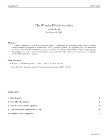
21THE ADM FORMALISMIntroductionIn short, we will reformulate general relativity (GR) in the (ADM or) Hamiltonian formalism by showing that the EinsteinHilbert action results from a Hamiltonian which only consists of two constraints: The diffeomorphism constraint Ha 0ˆaΨ 0and the Hamiltonian constraint H 0. After canonically quantising the spatial metric these two take the form Hˆ Ψ 0. The former is called the quantum diffeomorphism (or momentum) equation and the latter is named inand Hhonour of the work by Wheeler[4] and DeWitt[5] the Wheeler-DeWitt equation.The idea of quantising GR is one of many attempts to unify two of the most successful theories in theoretical physics.One of these theories is the standard model (SM). As a quantum field theory it describes the fundamental particles toa large success. Even though there are still severe open problems1 the discovery of the Higgs at the LHC in 2012 andthe success of the quark model are a clear indication that a grand unified theory (GUT) must to some extend describenature in a similar form. The other theory is GR. It has been tested and is tested every day describing nature not onlyon the astronomical scales but as the recent detection of the gravitational waves show also on much smaller scales (ofgravitational interaction). In fact this detection presents a first test in the very-strong field regime of GR and providesfurther evidence for the existence of black holes. Up to date it is an open question how to combine these two theories toa consistent description of nature at all scales.Even though the brute force quantisation of GR presented in the following sections is quite a drastic upshot and bringswith it numerous problems, it lead to a connection representation of GR, which ultimately lead to the development ofquantum loop gravity (QLG). Which is depending on whom one asks next to or after string theory one of the furthestdeveloped GUT at our hands.2The ADM formalismA revelation of the (ADM2 or) Hamiltonian formulation of GR is the separation of the Einstein Field equations Gµν Λg µν T µν into the time-independent equations of (or constraints on) the metric from the time dependent (or evolution equations)of the metric. This way the constraints describe the data one can encode on the metric and the evolution equations theirevolution w.r.t time. One speaks of the initial value formalism of GR. We will come back to this point after derivingthe constraints of GR. Bear in mind that for a canonical quantisation of GR the Hamiltonian description is needed tosubstitute the Poisson bracket with the commutator.2.1Foliation of spacetime and the ADM actionIn the ADM formalism of GR spacetime, a 3 1 dimensional Riemannian manifold M with metric g, is foliated 3 into aone parameter family or trajectory of space-like slices (leaves 3 ) {Σt t R} (see Figure 1). Unless otherwise noted we willassume the spatial slices to be closed4 .Each of these slices has the dynamical (ADM) variables:hab the metric tensor of the spatial slices induced by g (pullback of the ambient spacetime)c dpab their conjugate momenta (w.r.t. the poisson bracket, i.e. {hab (x), pcd (y)} δ(aδb) δ(x, y))Note that we will only introduce the ‘distinguished time’, induced by this background foliation, for the moment being.and workOn the one side of the coin we need this ‘distinguished time’ in order to define a conjugate momentum, p L q̇in an Hamiltonian formalism. While on the other side of the coin GR is background-independent. This means that thereis no background structure, ‘everything is relative’ or in this context: there is no absolute time. We will come back tothe discussion of background-independence in the Hamiltonian formalism after deriving it.1 Hierachyproblem, strong CP problem, .Richard Arnowitt, Stanley Deser and Charles W. Misner[6]3 see mathematically precise definition4 In the open case one can attribute asymptotic boundary conditions. These take the form of asymptotic boundary conditions with respectto (w.r.t.) an embedding into another manifold. However, such conditions imply that there is a part of the universe outside the region beingmodeled and since we consider GR to be a theory of the whole universe we shall restrict ourselves to the closed case.2 After2Page 2 of 13
2.1Foliation of spacetime and the ADM action2 THE ADM FORMALISMtimeMΣt′′Σt ′ΣtFigure 1: A foliation of a manifold M into spatial slices ΣtIn order to construct a Hamiltonian formalism we will not start with the tensorial form of the Einstein Field equationsGµν T µν but the Einstein-Hilbert action 16πGN SEH dtd3 x g(R 2Λ).MWith the background-independence of GR in mind we will express this action only in the ADM variables of the spatialslices, i.e. eliminate the time components5 .The heart of this step is Gauß famous theorema egregium (remarkable theorem) in 3 1 dimensions. The remarkable partof this theorem is that one can express the extrinsic curvature R of the spatial slice Σt given by the embedding spacetimeM only by intrinsic parameters, i.e. those which can be determined within Σt :R(1) Kab K ab K 2 (3) R.R is here the induced curvature within the spacial slice and Kab (x) 12 Ln hab (x) the Lie derivative of hab w.r.t. the(time-like) unit vector field nµ (x) orthogonal to the slices.One can show that there always exists a globally hyperbolic ‘time function’ tµ (x), i.g. not orthogonal to the slices, forthe foliation such that each slice is a Cauchy surface (constant in time tµ ; each point on the slice has the same timevalue). In other words the time arrow in Figure 1 just indicated the overall direction. The actual vector field tµ (x) cantake more arbitrary flows (see Figure 2).(3)timeMΣt′′Σt′Σtt′′µ (x)t′µ (x)tµ (x)Figure 2: An illustration of the ‘time function’ tµ (x) moving through a foliated manifold M for a fixed point x.Let us decompose this flow of time into components normal (nµ nµ 1) and tangential to Σt ,tµ (x) N (x)nµ (x) Nµ (x).We can see in Figure 3 that N (x) is the relative factor between the (absolute) time of the embedding space and theinduced time experienced by moving though the foliation and N a (x) describes how a fixed point in the spatial slice Σt isshifted in the embedding space to the same point in the next slice Σt dt . In short, the lapse function N (x) and the shiftfunction N a (x) describe how to move from slice to slice. In this sense we say that:5 By tracing the second Bianchi identity accordingly one can show that the 0ν components of the Einstein Field equations do not determinethe time evolution of the metric. In other words, we expect the 4 Einstein Field equations corresponding to the 0ν and ν0 entries to describethe constraints and the other 6 spatial entries to describe the time evolution. We can take this as a motivation to separate time from thespatial slices.3Page 3 of 13
2.2Recovering Background-independence2THE ADM FORMALISM Na generates spatial diffeomorphsims while ‘gliding’ through the foliation N generates pointwise change in the velocity with which one ‘glides’ through the foliationxΣt dtẊµ dtN (x)nµ dt xXµ,a N a (x)dtΣtFigure 3: An illustration of how the ‘time function’ tµ (x) maps points from one spatial slice Σt to the spatial slice of thenext instance Σt dt . Xµ are the coordinates of the embedding spacetime M. One can express the volume element g in terms of the induced metric h (see [1, Ch. 4]) g N h.(2)After inserting Equation 1 and Equation 2 in the Einstein-Hilbert action we get the ADM action: 16πGN SADM gR (thm. egregium)³¹¹ · ¹ µ ³¹¹ ¹ ¹ ¹ ¹ ¹ ¹ ¹ ¹ ¹ ¹ ¹ ¹ ¹ ¹ ¹ ¹ ¹ ¹ ¹ ¹ ¹ ¹ ¹ ¹ ¹ ¹ ¹ ¹ ¹· ¹ ¹ ¹ ¹ ¹ ¹ ¹ ¹ ¹ ¹ ¹ ¹ ¹ ¹ ¹ ¹ ¹ ¹ ¹ ¹ ¹ ¹ ¹ ¹ ¹ ¹ ¹ ¹ ¹ ¹ µdtd3 x N h ( Kab K ab K 2 (3) R 2Λ)MOne may think of Kab as the velocity field of hab (x) ‘gliding’ through the foliation. By defining the ‘DeWitt metric’Gabcd 2h (hac hbd had hbc 2hab hcd ) this action takes the form16πGN SADM dtd3 x N ( Gabcd Kab Kcd h ((3) R 2Λ) ).M ¹¹ ¹ ¹ ¹ ¹ ¹ ¹ ¹ ¹ ¹ ¹ ¹ ¹ ¹ ¹ ¹ ¹ ¹ ¹ ¹ ¹ ¹ ¹ ¹ ¹ ¹ ¹ ¹ ¹ ¹ ¹ ¹ ¹ ¶ ¹¹ ¹ ¹ ¹ ¹ ¹ ¹ ¹ ¹ ¹ ¹ ¹ ¹ ¹ ¹ ¹ ¹ ¹ ¹ ¹ ¹ ¹ ¹ ¹ ¹ ¹ ¹ ¹ ¹ ¹ ¹ ¹ ¹ ¹ ¹ ¹ ¹ ¹ ¹ ¹ ¶‘kin. term’(3)‘pot. term’The contribution of the ‘kinetic’ term to the action is determined by the ‘DeWitt metric’ Gabcd . We will postpone its1(ḣab Da Nb Db Na ), where Db is the covariant derivative6 ondiscussion and insert the exact expression for Kab 2N7Σ, into the ADM acton to rewrite it in the form :L16πGN SADM³¹¹ ¹ ¹ ¹ ¹ ¹ ¹ ¹ ¹ ¹ ¹ ¹ ¹ ¹ ¹ ¹ ¹ ¹ ¹ ¹ ¹ ¹ ¹ ¹ ¹ ¹ ¹ ¹ ¹ ¹ ¹ ¹ ¹ ¹ ·¹ ¹ ¹ ¹ ¹ ¹ ¹ ¹ ¹ ¹ ¹ ¹ ¹ ¹ ¹ ¹ ¹ ¹ ¹ ¹ ¹ ¹ ¹ ¹ ¹ ¹ ¹ ¹ ¹ ¹ ¹ ¹ ¹ ¹ µ dtd3 x ( pab ḣab N H g N a Hag )M ¹¹ ¹ ¹ ¹ ¹ ¹ ¶ ¹¹ ¹ ¹ ¹ ¹ ¹ ¹ ¹ ¹ ¹ ¹ ¹ ¹ ¹ ¹ ¹ ¹ ¹ ¹ ¹ ¹ ¹ ¹ ¹ ¹ ¹ ¹ ¹ ¹ ¹ ¹ ¹ ¹ ¹ ¹ ¹ ¹ ¹ ¹ ¹ ¶‘pv ′(4) Hg (‘constraints’)with H g 16πGN Gabcd p pHag 2Db pa b .ab cd h (3)( R 2Λ)16πGNIt should be worth mentioning that in the presence of Yang-Mills fields H g gets an additional contribution H Y M , i.e.H g H g H Y M (see [1, Ch. 4.1] for a derivation).2.2Recovering Background-independenceThe diffeomorphism- and Hamiltonian constraintRecall that GR is background-independent and therefore the information of the (fixed background) foliation encodedin the lapse- and shift functions N and N a can be arbitrary functions. By varying Equation 4 w.r.t to N or N a and6 D T b1 .brac1 .cs 7 For a step-by-stephda hbe11 .hberr hcf1 .hcfs d T e1 .er f1 .fs (hda ‘projects onto’ Σ)s1discussion see [1, Ch. 4]4Page 4 of 13
2.2Recovering Background-independence2THE ADM FORMALISMdemanding that the expression vanishes, we get the Hamiltonian- or momentum (or diffeomorphism) constraint:H gHag 0 0(Hamiltonian constraint)(momentum- or diffeomorphism constraint).This ensures, independently on how N and N a vary (i.e. the spacial slices evolve in time), that these constraints and thusthe Einstein Field equations be fulfilled at all events. And just as important, it ensures that we recover the backgroundindependence of GR, since N and N a are now the Lagrange multipliers of the constraints.With this in mind let us carefully distinguish between the foliation {Σt t R} of some Riemannian manifold M and thespatial slice Σ we are evolving in time by mapping it into or perhaps in a more intuitive sense ‘gliding though’ this foliation(see Figure 4). It is crucial to arrive at this distinction to recover the background-independent picture.timeMΣt′′t′′t′t′′µ (x)t′µ (x)Σt ′ΣtΣttµ (x)Figure 4: Mapping a spacial slice Σ through a foliation of a manifold MTime in the ADM formalismThe ADM formalism is by construction in the 3 1 decomposition of GR and therefore its time evolution as a Hamiltoniansystem is given by the Poisson bracket and the HamiltoniandF (x)dt {F (x), Hg (x)}P.B. F (x). tThis, however, is the evolution of ‘gliding’ through the foliation and therefore not background-independent. More precisely,we saw in the previous subsection that in this Hamiltonian form of GR the choice of time is fixed by ‘pinning down’points to any background structure. To regain background-independence we separated the spatial slice Σ from foliationof some manifold.Now we are left with the problem of finding a background-independent way of recovering a time for our theory. In thissense the demand for background-independence in the ADM formulation reveals a timeless 8 aspect or redundancy of thechoice of time at the classical level.In the attempt to find a possible solution to this problem we will first draw a parallel between the ADM formulationand electrodynamics as initial value formalisms and then see to what extend GR is a relational theory9 . The latter willshow us whether one can reconstruct, given the right information, a time form the three-dimensional geometry of twoconfigurations (slices).Time in a relational systemThe Hamiltonian of GR consisted only on the (time-independent) Hamiltonian- and momentum constraints. The corresponding equations in classical electromagnetism (EM) are the time-independent Maxwell equations. Likewise the timeevolution of the foliation corresponds to the time-dependent equations10 .8 For aspects of timelessness in classical dynamics see the beautifully written essay of J. Barbour [8] in which he is surprisingly pleased withthe idea of a timeless theory. For a more detailed and closer discussion w.r.t. GR see [1, Ch. 3.4].9 Space or time is defined as relationships among events.10 Note that one can use the 4 degrees of freedom (d.o.f.) of the constraints to fix 4 of the 6 d.o.f. of the evolution equations of the spatialslices. The remaining 2 d.o.f. can in the transverse traceless gauge be identified with the x and polarisations of the weak-field expansion ofthe gravitational field.5Page 5 of 13
2.2Recovering Background-independence2ADM formulation of GRtime independent eq. of motion(hold at all times)H and Ha (4 d.o.f.)time dependent eq. of motion(evolution in time)evolution of hab(6 d.o.f.)(‘gliding’ through the foliation)THE ADM FORMALISMclassical EM⃗⃗ E ⃗⃗ B⃗ E⃗ B 4πρ 0⃗ 4π⃗j⃗ B ⃗⃗ E In electrodynamics specifying the B-field on two hypersurfaces is not sufficient, additionally one needs to fix the timeparameters of the two hypersurfaces. Therefore, in the case of our timeless version of the ADM formulation we wouldexpect additionally to the configurations of two spatial slices (Cauchy surfaces) the corresponding times. With this inmind, there is the so called ‘sandwich conjecture’ (see Figure 5), which states that one can always determine the temporalseparation between two slices. There is also the (stronger) infinitesimal version of this conjecture, the ‘thin-sandwichconjecture’ (formulated by [7]), which only needs the spatial metric and the infinitesimally propagating direction in phasespace to determine the temporal evolution of hab .But is the ‘sandwich conjecture’ enough to predict the future evolution of the slices? There is not much known. However,in the classical Newtonian case one cannot predict the future evolution by two such successive ‘pictures of the universe11 ’,since one lacks the information of the angular momentum and kinetic energy of the system. This is the so called ‘Poincarédefect’[10]. A way around this problem has been developed by Barbour and Bertotti [11] by introducing a ‘gauge freedom’w.r.t. translations and rotations and then ‘fixing this gauge’ (see [1, Ch. 3.4]). We will see an analog in going to theconnection representation of GR by replacing the metric field with a dreibein invariant under rotations. But lets not getahead of ourselves.If the two times of these configurations or its the relative speed is given and we neglect the ‘Poincaré defect’, one candetermine the future evolution from the two configurations in the relational system. Barbour goes a step further andargues for a completely timeless model in which ‘time can be read off the heaven’ by taking successive snapshots of theuniverse. For a classical example see his essay [8]. He pursuits to develop a completely timeless description of the universein which only ‘shapes12 ’ physically matter. Its important to stress that this is only one of many speculative directionsand not widely accepted. y′](′](,Σ,ΣΣΣ t[ t[Σxx)y)Σ′ yxFigure 5: Illustrating the ‘sandwich conjecture’.The question whether space is an absolute- or relational structure dates back to Aristotle, Descartes, Newton13 , Leibnitz,Mach and many more. But is GR itself a relational system? Not completely, only when we mod out the diffeomorphismsof GR a relational physical theory is recovered [9]. W.r.t. the question of background-independence it is worth having acloser look at Einsteins struggle with the general covariance of GR in Appendix A (we closely followed [3, Ch. 2.2.5]).In the ADM formalism our parameter space consisted of the foliation and the ADM variables. Since the momentumwas defined using the distinguished time of the foliation our parameter space of the background-independent timelesspicture only consists of the set of spatial (pseudo-)Riemannian metrics Riem(hab ). In the coming subsection 2.3 we willidentify the metrics related by diffeomorphisms and discuss the resulting quotient space, called ‘superspace’. Let us nowsummarise our attempt so far to recover background-independence from the ADM formalsm.11 consistingof a collection of point-massesin triangles, matter ratios,. (see http://www.platonia.com/research.html)13 Part of the critique of Newtons concept of space as an absolute structure comes from his introduction of an absolute space. Furthermore,for Newton time as a parameter was introduced for the purpose of solving his differential equations. In this sense it was a mathematical trick.However, Einsteins development of GR introduced a background-independent theory. For an in depth discussion we will direct the reader toRovelli’s wonderful book [3, Ch. 2.2 especially Ch. 2.2.2 & 2.2.5], once again Barbours essay [8], [1, Ch. 3.4] or [9].12 Angles6Page 6 of 13
2.3Superspace and the ‘De-Witt metric’2THE ADM FORMALISMSummaryWe started reconstructing the background-independent picture form the ADM action by varying the lapse- and shiftfunction. Their resulting equation of motions (eom) are called the Hamiltonian- and momentum-constraint and completelymade up the Hamiltonian of GR. Consequently, we had to distinguish between the spatial slices of the background-manifoldand the separated spatial slice which we evolved through the foliation. Arriving at a what appears to be timeless threedimensional picture.Motivated by Einsteins struggle with the general covariance of GR, we proceeded by identifying diffeomorphic spatialslices. This way we retrieved GR as a timeless relational system which is still background-independent. In such a systemtime-evolution can be recovered by ‘taking successive pictures of the universe’, i.e. two spatial slices, provided that wehave, in analogy to the electromagnetic example, the times of both (Cauchy surfaces) and neglect the ‘Poincaré defect’.In order to not to go down into too recent and speculative paths we left the reader at this point.2.3Superspace and the ‘De-Witt metric’SuperspaceIn order to gain a relative system we argued in the previous subsection to mod out the diffeomorphisms of our spatialslice Σ. Therefore instead of considering the whole configuration space14 of spatial (pseudo-)Riemannian metrics hab ofΣ we identify metrics related by a diffeomorphism and form the quotient space:S(Σ) Riem(Σ)/Diff(Σ).This space was introduced by Wheeler as superspace 15 .The ‘De-Witt metric’In fact, the ‘De-Witt metric’ we introduced in Equation 3 plays the role of a metric on Riem(Σ). Due to its symmetry itcan be considered to be a 6 6 matrix which maps two (symmetric) mertrics lab , kcd tangent to a point hab in Riem(Σ)to a real number.G(l, k) d3 x Gabcd lab kcd .ΣIt might be useful to note that the ‘DeWitt-metric’ has the same symmetries as an elasticity tensor. After diagonalisationone finds that it is of Lorentzian signature( , , , , , ),which makes it an indefinite metric. Recall that the ‘De-Witt metric’ describes the kinematic term of the ADM Lagrangian(Equation 3), consequently one can show that its indefinite sign determines whether gravity acts as a attractive- orrepulsive force (see [1, Ch. 4.2.5]). Therefore, this metric governs the dynamics of GR in the ADM formalism.It is worth pointing out, in the premises of the connection representation of GR, that if we would use left-handed triadsinstead of metrics, the minus sign would necessarily flip one left-handed triad to a right handed one. A metric doesn’tkeep track of such handedness.So far so good, but is the metric also a metric on superspace? In superspace we cannot distinguish between the ‘vertical’direction along the orbits of diffeomorphic metrics and the ‘horizontal’ direction orthogonal to it (see Figure 6). This iswhere the indefinite property of the ‘De-Witt metric’ becomes troublesome, since in the ‘light-like’ case of zero norm thevertical- and horizontal (‘light- and space-like’) subspaces overlap. Consequently, the ‘De-Witt metric’ is only a metricon the ‘time- and space-like’ sectors.14 Additionally one can include the foliation of a background manifold in the configuration space and the configuration space of the matterfields.15 Not to be confused with the superspace of supersymmetry (SUSY).7Page 7 of 13
3THE WHEELER-DEWITT EQUATIONFigure 6: An illustration (taken from[1, Ch. 4.2]) of projecting orbits ofdiffeomorphic metrics in Riem(Σ) topoints in superspace. The cones indicate the Lorentzian ‘De-Witt metric’.h lies in the time-like sector, h′ on thelight-like sector and h′′ in the spacelike sector. The point [h′ ] lies on aborder between the time- and spacelike sectors in superspace. The ‘DeWitt metric’ is not a metric at pointsof such borders.Propagating in superspace instead of Riem(Σ) ensures that we only propagate between different physical solutions ofthe background-independent formalism of GR. Loosely speaking we modded out the ‘gauge group’ of GR and are leftwith such ‘light- and space-like’ sectors. Again, to recover background-independence, as we tried in the previous section,we are left with the timeless picture. One could either keep a timeless picture or ‘fix a time’ either before or afterquantisation. Note that time evolution doesn’t necessarily imply to ‘propagate from one point in superspace to another’.Instead time evolution may also be realised through a topological change of superspace (see Figure 7). But, topologychanging spacetimes come already at the classical level with severe problems such as singularities, closed time-like curvesand degenerate metrics[2]. Consequently, there is much room for speculation and we are left again with a questionableproposition.Figure 7: An illustration of ‘growing anose’ on a superspace Σi (taken from [2]).Note that, the structure of the superspaceS(Σ) is in general of a more complicatedform than Riem(Σ). Furthermore, recallthat we restricted ourselves to compactslices.3The Wheeler-DeWitt equationIf we knew what it was we were doing,it would not be called research, would it?- Albert EinsteinThe quantisation of an Hamiltonian system is at the mathematical level a straight forward procedure: In the case of theHamiltonian formalism of GR we promote hab and pcd to operatorsĥab (x)Ψ[hab (x)] hab Ψ[hab (x)]̵ δhp̂cd (x)Ψ[hab (x)] Ψ[hab (x)]i δhcdand replace the Poisson bracket with the usual commutation relations[ĥab (x), p̂cd (y)]̵ c δ d δ(x, y). ihδ(a b)8Page 8 of 13
3THE WHEELER-DEWITT EQUATIONThe highly non-trivial part is actually make sense of what we are doing. Ψ[hab (x)] is here a wave functional and its notclear where its living in. We will implement the constraints according to Dirac: hδ22̵ˆ((3) R 2Λ) )Ψ[hab (x)] 0H Ψ[hab (x)] ( 16πGN h Gabcd δhab δhcd 16πGN̵ˆ a Ψ[hab (x)] ( 2Db Hac h δ )Ψ[hab (x)] 0.Hi δhbcThe first of these two functional equations is called the Wheeler-DeWitt equation and the second is called the quantumdiffeomorphism equation. Sometimes one refers to both as the the ‘Wheeler-DeWit equations’. There are many problems16with regard to the Wheeler-DeWit equations. A central one is that one can not define[1, Ch. 5.2.2] a suitable measurefor a Schrödinger-type inner-product⟨Ψ1 Ψ2 ⟩ Riem(Σ)Dµ[h] Ψ 1 [h]Ψ2 [h].Hence, such a construction is at most formal. Also note that the ‘DeWitt metric’ explicitly appears in the Wheeler-DeWittequation. Therefore the discussion of superspace is also vital after canonical quantisation.We will now turn to the famous problem of time in quantum gravity (QG) and then proceed to the connection representation.The problem of timeIn quantum mechanics (QM) time is an absolute parameter governing the evolution of states:̵ Ψ.ˆHΨ ih tBut GR is background-independent and cannot depend on an absolute time. In fact, we demand by backgroundindependence that the l.h.s., the Hamiltonian, vanished upon acting on the wave functional (for an empty universe).A consistent theory of QG should therefore exhibit a novel concept of time. This is called the problem of time. Asmentioned before, to fix this problem we are left with the cases of considering a timeless model, fix a time before- or afterquantisation. There is much speculation concerning each of these paths. At last we once again point out that the role oftime in QG is not clear. Quoting Smolin[9]:‘The issue [the problem of time] is controversial and there is strong disagreement among experts. [.] The problem oftime is a key challenge that any complete background independent quantum theory of gravity must solve.’In the case of our canonical quantisation of the ADM formalism, time and therefore spacetime is absent in the ‘WheelerDeWitt equations’. Only the spatial metric has survived in the argument of the wavefunctional, whose embedding spaceis not clear. Time as well as probability are both left in this formalism as phenomenological concepts.A way to think of this phenomenon is to draw the analogy to the disappearance of trajectories in quantum mechanics thattime here disappeared from space-time. From this perspective the wavefunctional would smears out metrics in superspace,in the same sense as it usually smears out paths in space. Consequently, a sum over paths would corresponds to a sumover histories.Change of parametersTo solve the central Wheeler-DeWitt equation presented above three choices of variables have been developed: Quantum-Geometrodynamics with variables: three-metric and the extrinsic curvature Connection dynamics with variables: a connection Aia and a non-abelian electric field Eia Loop dynamics: variables connected by holonomies with Aia and the Flux of EiaWe will now briefly present the connection formulation of GR and comment on a solution of the corresponding quantumWheeler-DeWitt equations.16 Fora overview see [1, Ch. 5.2].9Page 9 of 13
44THE CONNECTION FORMULATION OF GRThe connection formulation of GRThe Ashtekar variablesIn the connection formulation of GR we replace the usual gravitational field of the ADM formalism17 given by the(spatial-)metric gab (x) with a triad (Dreibein) Eia (x) h(x)eai (x).(5) iwith h(x) det(ea ) . By using these so called Ashtekar variables we added a freedom or orientation and handedness18to the gravitational field which varies from point to point in space (see Figure 8). In other words, using the Ashtekarvariables 5 the gravitational field takes the form of a non-abelian vector field with gauge-group SO(3) or its double coverSU (2) (with an additional handedness). To promote this additional gauge freedom to a local property we introduceadditionally to the Levi-Civita connection Γi jk the corresponding spin connection ωa i j Γi jk eka of the gauge-groupDa eib a eib Γc ab eic ωa i j ejb .From the orthogonality condition of the triad:hab eai ebj δijone can recover the local (inverse) metrichab eai ebi .One may think of the local rotational d.o.f. of the triad as an intrinsic spinorial d.o.f. of a field. In fact, when Ashtekarformulated this connection representation he was influenced by Penroses Twistor theory and therefore first chose thegauge group SU (2). In this comparison the spin corresponds to the orientation of the triad in the embedding space.Figure 8: Illustrating triads in spacetime. The reader should be aware that the local triad is the gravitational background.In this sense this picture is not background-independent. We already arrived at a formulation which are not fields inspacetime, but fields on fields.Analogously to the familiar spinorial case we define the object:1Γia ωajk ijk ,2which describes the rotation δω i of parallel transporting a vector v i (see Figure 9) throughδω i Γia dxadv i i jk v i δω k .v′v′′vFigure 9: Parallel transport of a vector along a rotating triad.17 There18 Left-is also a vierbein formalism for the common formulation, see [3, Ch. 2]or right-handed field10Page 10 of 13
4THE CONNECTION FORMULATION OF GRLet us proceed by introducing a new variableKai Kab ebi .Kab is here the second fundamental form of the spatial slice. One can shown thatKai δE ia 8πGN pab δhab .in other words Kai is the canonically conjugate momentum of Eia . By going to the triad formulation we ended up with 9d.o.f. for each triad and need to fix the gauge this is done by imposing the constraint ijk Kaj E ka 0.It is called as the Gauß constraint and ensures that the angular momentum vanishes ‘p x 0’. The 9 d.o.f. of the triadeai are now reduced to the 6 d.o.f. of hab .The connection AiaAshtekars central step consisted in combining Eia and Kai into a complex connection AiaGN Aia Γia βKai ,where β is the ‘Barbero-Immirzi’ parameter. The crucial property of our new connection Aia is that it is the canonicallybconjugate variable of Ej/8πβ :{Aia (x), Ejb (y)} 8πβδji δab δ(x, y).P.B.In addition one has:{Aia (x), Ajb (y)} 0.P.B.The associated curvature isiFab 2GN [a Aib] G2N ijk Aja Akb .The Hamiltonian constraints take for β i and Λ 0 the fo
CONTENTS CONTENTS The Wheeler-DeWitt equation Matías Hersch February 10, 2017 Abstract: T