Transcription
9.07 Introduction to Statistics for Brain and Cognitive SciencesEmery N. BrownLecture 11: Monte Carlo and Bootstrap MethodsI. ObjectivesUnderstand how Monte Carlo methods are used in statistics.Understand how to apply properly parametric and nonparametric bootstrap methods.Understand why the bootstrap works.“John Tukey suggested that the bootstrap be named the shotgun, reasoning that it could blowthe head off any statistical problem if you were willing to tolerate the mess.”Paraphrased from Efron (1979).“Dad, I just freed my mind!”Elena Brown, 5 years old, explaining to me the secret of how she got control of her skis andsuccessfully negotiated the bottom third of the ski slope on her first run of the new ski season.II. Monte Carlo MethodsComputer simulations are useful to give insight into complicated problems when detailedanalytic studies are not possible. We see this all the time in physics, chemistry, climatology andecology, just to cite a few examples. Because by definition, stochastic simulations introducerandomness in to the study, they are often referred to as Monte Carlo methods after the capitalcity of the principality of Monaco, which is known for gambling. We have already made use ofMonte Carlo methods to check the theoretical properties of some of our statistical proceduressuch as confidence intervals in Lecture 8, and to compute posterior probability densities in ourBayesian analyses in Lecture 10 and in Homework Assignment 7.In this lecture, we will present a very general, computer-intensive method called the bootstrapto compute from a random sample an estimate of a particular function of interest and theuncertainty in that function. The bootstrap was first proposed by Brad Efron at Stanford in 1979(Efron, 1979). Since then it has become one of the most widely-used statistical methods. As hasoften been the case for Monte Carlo methods in general, it has made it possible to solve easilya number of estimation problems that would not have been possible or certainly far more difficultby other means. We begin by reviewing two elementary Monte Carlo methods.A. Inverse Transformation Method. Before beginning with the bootstrap, we re-present one ofthe most basic Monte Carlo algorithms for simulating draws from a probability distribution. A cdfF outputs a number between 0 and 1. Therefore if F is continuous and if we take U as auniform random variable on (0,1), then we can defineX F 1 (U )(11.1)where F 1 (u ) equals x whenever F ( x) u. Because F ( x) is continuous and monotonic, it followsthat we can simulate a random variable X from the continuous cdf F, whenever F 1 iscomputable by simulating a random number U , then setting X F 1 (U ). These observationsimply the following algorithm known as the Inverse Transformation Method.
page 2: 9.07 Lecture 11: Monte Carlo and Bootstrap MethodsAlgorithm 11.1 (Algorithm 3.1, Inverse Transformation Method)Pick n large.1. For i 1 to n.2. Draw U i from U (0,1) and compute X i F 1 (Ui )3. The observations ( X1,., X n ) are a random sample from F.Example 3.2. Simulating Exponential Random Variables (Revisited). In Lecture 3, wedefined the exponential probability density asf ( x) λ e λ x(11.2)for x 0 and λ 0. It follows that the cdf F ( x) isF ( x) x 0 λe λudu 1 e λ x .(11.3)To find F 1 (u ) we note that1 e λ x ux log(1 u)λ(11.4)(11.5)Hence, if u is uniform on (0,1) thenF 1 (u ) log(1 u)λ(11.6)is exponentially distributed with mean λ 1. Since 1 u is uniform on (0,1) , it follows thatlog(u )is exponential with mean λ 1. Therefore, we can use Algorithm 3.1 to simulatex λdraws from an exponential distribution by using F 1 in Eq. 11.6.B. Sampling from an Empirical Cumulative Distribution Function. The same idea we usedto simulate draws from a continuous cdf may be used to simulate draws from a discontinuous orempirical cdf. That is, given x1,., xn define the empirical cumulative distribution function asnFn ( x) I {xi x}i 1n(11.7)
page 3: 9.07 Lecture 11: Monte Carlo and Bootstrap Methodswhere I {xi x} is the indicator function of the event xi x for xmin x xmax . We have that Fn ( x)is the cdf corresponding to the empirical probability mass function that places weight1at everynobservation. We can express the empirical cdf alternatively as 0 x x(1) kFn ( x) x( k ) x x( k 1) n 1 x( n) x (11.8)where the x(i ) are the ordered observations or order statistics from i 1 to n andnk I {xi x}.Remember we use the order statistics to construct the Q-Q plots. We definei 1Fn 1 (u ) asFn 1 (u ) x(k )if(11.9)kk 1for k 1,., n 1. u nnAn example of an empirical cdf is shown in Figure 11A which shows the retinal ISI data fromExample 8.1. There are 971 observations here so that the jump of1at each order statisticncorresponds to a jump of approximately 10 3. For this reason, this empirical cdf looks verysmooth.
page 4: 9.07 Lecture 11: Monte Carlo and Bootstrap MethodsFigure 11A. Empirical Cumulative Distribution Function for Retinal ISI Data (Example 8.1).Remark 11.1. Fn ( x) is an estimate of the unknown cumulative distribution function F ( x). Thiscan be justified by the Law of Large Numbers (Lecture 7) and more strongly by anotherimportant result in probability theory called the Glivenko-Cantelli Lemma. This lemma saysthat as n goes to infinity Fn ( x) converges uniformly to the true F ( x) in distribution.Note on Notation. In our lectures we have used θ to denote the parameter in our probabilitymodels. In this lecture we represent this parameter by ξ in order to let θ , as we show belowdefine the generic function whose properties are characterized in a bootstrap analysis.Remark 11.2. In Lectures 8 to 10 we studied method-of-moments, likelihood and Bayesianmethods for estimating the parameters of probability models. In each case, we wrote down aspecific probability model to describe the data and used one of these three approaches toestimate the model parameters. These models, such as the binomial, Poisson, Gaussian,gamma, beta and inverse Gaussian are parametric models because given the formula for theprobability distribution, each is completely defined once we specify the values of the modelparameters. In this regard our method-of-moments, likelihood and Bayesian methods providedparametric estimates of the probability distributions. That is, given a probability distributionxf ( x ξ ) the associated cdf is F ( x ξ ) f (u ξ )du. Hence, given ξˆ an estimate of the parameter xξ we have that F ( x ξˆ) f (u ξˆ)du is the parametric estimate of the cdf is F ( x ξˆ). Therefore, given F ( x ξˆ), we can use Algorithm 3.1 to simulate estimated samples from F ( x ξ ). The typeof optimality properties of F ( x ξˆ) and the samples from it will follow from the optimalityproperties of the type of estimation procedure used to compute ξˆ.Remark 11.3. In contrast to F ( x ξˆ) in Remark 11.2, we term the empirical cumulativedistribution function Fn ( x) a nonparametric estimate of F ( x). This is because we can computeit without making any assumption about a specific parametric form of F ( x). Just as we can useAlgorithm 3.1 applied to F ( x ξˆ), to simulate estimated samples from F ( x ξ ), we can use F ( x)nto simulate samples from F ( x). The prescription is given in the next algorithm.Algorithm 11.2 (Sampling from an Empirical Cumulative Distribution Function).Pick n* .1. For i 1,., n*2. Draw U i from U(0,1).3. Compute X i* Fn 1 (Ui ) in Eq. 11.9.The sample (X1* ,., X n* ) is a random sample from Fn ( x).
page 5: 9.07 Lecture 11: Monte Carlo and Bootstrap MethodsThe parametric and nonparametric estimates of the cdf are the key tools we will need toconstruct the bootstrap procedures.III. Bootstrap Methods (Efron and Tibshirani, 1993; DeGroot and Schervish, 2002; Rice2007).A. Motivation.To motivate the bootstrap we return to two problems we considered previously.Example 8.1 (continued). Retinal Neuron ISI Distribution: Method-of-Moments. In thisproblem, we have been studying probability models to describe the ISI distribution of a retinalneuron. One of the models we proposed for these data was the gamma distribution withunknown parameters α and β . We found that the method-of-moments estimates wereβˆMM X (σ̂ 2 ) 1(11.10)α̂ MM X 2 (σ̂ 2 ) 1.(11.11)One of the points we made in Lecture 8 was that while we could find approximations to thedistributions of X using the central limit theorem and that of σˆ 2 under the special assumption ofGaussian data, it was in general difficult to find the distribution of the sample moments andfunctions of these moments. However, this is exactly what we need in order to determine theuncertainty in the method-of-moments estimates of α and β in Eqs. 11.10 and 11.11.Example 8.1. (continued). Retinal Neuron ISI Distribution: Five-Number Summary. One ofthe first things we did to analyze these data was to compute the five-number summary inLecture 8 (See Figure 8B). These are the minimum 2 msec, 25th percentile 5 msec, median(50th percentile) 10 msec, the 75th percentile 43 msec and the maximum of 190 msec. Each ofthese is a statistic and each estimates respectively, the true minimum, 25th percentile, median(50th percentile), 75th percentile, maximum. Hence, because each is a statistic, each hasuncertainty. Each of these is a nonparametric estimate of the corresponding true function of thedistribution. Suppose we wish to compute nonparametric estimates of the uncertainty in thesestatistics. None of the method-of-moments, likelihood or Bayesian theory we have developedwould allow us to compute the uncertainty in these estimates. Indeed, the analytics necessaryto study these estimates falls under the heading of the quite advanced areas of mathematicalstatistics called order statistics (Rice, 2007) and robust estimation theory (DeGroot andSchervish, 2002).These two problems can be generally formulated as follows. Suppose we have a randomsample x ( x1, ., xn ) from an unknown probability distribution F and suppose we wish toestimate the quantity of interest θ T ( F ( x)). The quantity θ can be either a parameter of aparametric probability distribution, or a nonparametric quantity, such as one of the componentsof the five-number summary. Suppose we estimate θ as θˆ T ( Fˆ ( x)) . How can we compute theuncertainty in θˆ ?B. The Nonparametric BootstrapBootstrap methods depend on the concept of a bootstrap sample. Let F̂ be an empirical cdf asdefined in Eq. 11.8. It puts mass 1/ n at every observation xi for i 1,., n. A bootstrap sample
page 6: 9.07 Lecture 11: Monte Carlo and Bootstrap Methodsis a random sample of size n drawn from F̂ which we denote as x* ( x1* , ., xn* ). We use the * toindicate that x* is not the actual data set x . Alternatively stated, the bootstrap sample x1* ,., xn*is a random sample of size n drawn with replacement from the set of n objects x1 ,., xn . Thebootstrap sample x1* ,., xn* consists of members of the original sample some appearing, zerotimes, some appearing once, some appearing twice, etc. Given a bootstrap sample, we cancompute a bootstrap replication of θˆ T ( Fˆ ( x)) defined as.θˆ* T ( Fˆ ( x*))(11.12)The quantity in Eq. 11.12 comes about by applying the function T to the bootstrap sample. Forexample, for the method-of-moments in Eqs. 11.10 and 11.11*βˆMM X * (σ̂ 2* ) 1(11.13)*α̂ MM X 2* (σ̂ 2* ). 1(11.14)In the case of the five-number summary, it would be the five-number summary computedat the bootstrap sample x1* ,., xn* .It follows that we can compute the uncertainty in θˆ T ( Fˆ ( x)) by simply drawing a largenumber of bootstrap samples, say B, from F̂ and we compute θˆ* T ( Fˆ ( x*)) for each sample. Ahistogram of θˆ* shows the uncertainty in θˆ. We could also summarize the uncertainty in θˆ bycomputing the standard error of the bootstrap replicates defined as1B 2* 1** 2ˆˆseB (θ ) ( B 1)(θb θ ) b 1 (11.15)where.θ * B 1B θˆ*b .(11.16)b 1Notice here we divide by B 1 instead of B because for many problems only a small number ofbootstrap replicates is required to accurately establish the uncertainty. The quantity θ * in Eq.11.16 is the bootstrap estimate. Dividing by B 1 provides an unbiased estimate of the standarderror. We could also compute an empirical 95% confidence interval based on the histogram ofthe bootstrap replicates. We term the procedure of drawing random samples with replacementfrom the empirical cdf F̂ to compute the uncertainty in θˆ a nonparametric bootstrapprocedure. The procedure is nonparametric because we use the nonparametric estimate of Fdefined in Eq. 11.8. We can state this in the following algorithm.Algorithm 11.3 (Nonparametric Bootstrap)Pick B.
page 7: 9.07 Lecture 11: Monte Carlo and Bootstrap Methodsˆ where x*b (x*b ,., x*b ) is a vector of1. Draw x*1,., x*B independent bootstrap samples from F,1nn observations which contains the b th bootstrap sample for b 1,., B.2. Evaluate the bootstrap replication corresponding to each bootstrap sample θˆ* (b) T ( Fˆ ( x*b ))for b 1,., B.3. Compute the uncertainty in θˆ as either the:i. sample standard error as seB (θˆ* ) defined in 11.15ii. histogram of the θˆ* (b) T ( Fˆ ( x *b ))iii. 95% confidence interval from the histogram.Remark 11.4. Notice that in the case of the method-of-moments estimates of the parameters ofthe gamma distribution, even though the functions of interest are parameters, we are using anonparametric bootstrap procedure to estimate their uncertainty.C. The Parametric BootstrapSuppose as in Remark 11.2 that given our random sample x1 ,., xn we estimate F not by theempirical cdf F ( x) but by a parametric estimate of the cdf F ( x ξˆ) using a method-of-momentsnor likelihood approach. Therefore, it follows that we can carry out our bootstrap procedure usingF ( x ξˆ) instead of the empirical Fn ( x) as the estimate of F . We term this procedure of drawingrandom samples with replacement from the parametric cdf Fˆ F( x ξˆ) to compute theuncertainty in θˆ a parametric bootstrap procedure. We can state this procedure formally inthe following algorithmAlgorithm 11.4 (Parametric Bootstrap)Pick B.1. Draw x*1,., x*B independent bootstrap samples from Fˆ F ( x ξˆ), where x*b (x1*b ,., xn*b ) is avector of n observations which contains the bth bootstrap sample for b 1,., B.2. Evaluate the bootstrap replication corresponding to each bootstrap sample θˆ* (b) T ( Fˆ ( x *b ))for b 1,., B.3. Compute the uncertainty in θˆ as either the:i. sample standard error as seB (θˆ* ) defined in 11.15ii. histogram of the θˆ* (b) T ( Fˆ ( x *b ))iii. 95% confidence interval from the histogram.Remark 11.5. An important difference between the nonparametric and parametric bootstrapprocedures is that in the nonparametric procedure, only values of the original sample appear inthe bootstrap samples. In the parametric bootstrap, the range of values in the bootstrap sampleis the entire support of F. For example, in the case of the retinal ISI data, there are 971 values.Therefore a nonparametric bootstrap procedure applied to these data would have only 971different values in any bootstrap sample. In the parametric bootstrap of this problem using the
page 8: 9.07 Lecture 11: Monte Carlo and Bootstrap Methodsgamma distribution the values in the bootstrap sample could be any value between zero andpositive infinity.Remark 11.6. We can use the parametric bootstrap to analyze the uncertainty in thenonparametric estimators such as the five-number summary.D. Applications of the Bootstrap1. Example 8.1 (continued) Nonparametric and Parametric Bootstrap Analyses of theMethod-of-Moments Estimates for the Gamma Distribution Parameters.We used Algorithms 11.3 and 11.4 to perform nonparametric and parametric bootstrapanalyses in order to estimate the uncertainty in the method-method of-moments estimates forthe gamma probability density parameters for the retinal ISI data. The histograms of theanalyses are shown in Figures 11B and 11C for α̂ MM and in Figures 11D and 11E for β̂MM .The findings from the analysis are summarized in Tables 11.1 for α̂ MM and 11.2 for β̂MM .Nonparametricα̂ MM0.6284α̂ B0.6299biasMM αˆ MM αˆ B-0.0015se(αˆ B )0.028195% 52(0.5437,0.7211)Table 11.1 Comparison of Nonparametric and Parametric Bootstrap Analyses of α̂ MM .Figure 11B. Histogram of nonparametric bootstrap samples of α̂ MM .
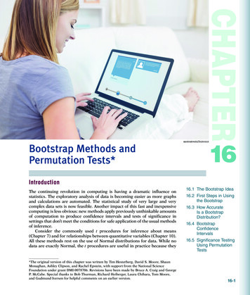
page 9: 9.07 Lecture 11: Monte Carlo and Bootstrap MethodsFigure 11C. Histogram of parametric bootstrap samples of α̂ MM .The parametric and nonparametric bootstrap estimates of α agree and both procedures showlittle to no bias (Table 11.1 column 3). The parametric bootstrap procedure has a largerstandard error and a wider 95% confidence interval (Table 11.1 columns 4 and 5) suggestingthat there is greater uncertainty in the estimate of α than suggested by the nonparametricanalysis.β̂ B0.0205biasMM βˆMM βˆB0.0001se(βˆB )0.000795% CINonparametricβ̂ 0.0239)(0.0191,0.0218)Table 11.2 Comparison of Nonparametric and Parametric Bootstrap Analyses of β̂MM .
page 10: 9.07 Lecture 11: Monte Carlo and Bootstrap MethodsFigure 11D. Histogram of nonparametric bootstrap samples of β̂MM .Figure 11E. Histogram of parametric bootstrap samples of β̂MM .Similarly, the parametric and nonparametric bootstrap estimates of β agree (Table 11.2) andboth procedures show little to no bias (Table 11.2, column 3). The parametric bootstrap hereas well suggests that there is greater uncertainty in the estimate of β than suggested by thenonparametric analysis (Table 11.2, column 4 and 5).2. Example 8.1 (continued) Nonparametric Bootstrap of the 75th Percentile.
page 11: 9.07 Lecture 11: Monte Carlo and Bootstrap MethodsFigure 11F . Histogram of Nonparametric Bootstrap samples of 75th Percentile.Nonparametric75th Estimate4375thB43.73bias75th 75th 75thB0.73se(75thB )5.1295% CI(33.6953.77)Table 11.3 Nonparametric Bootstrap Analyses of 75th Percentile.We used Algorithms 11.3 to perform nonparametric bootstrap analysis of the uncertainty in theempirical (order statistic) estimate of the 75th percentile. The histogram of the analyses is shownin Figure 11F and the findings from the analysis are summarized in Table 11.3. The orderstatistic and bootstrap estimates agree indicating that there is very little bias. The standard errorand 95% confidence intervals suggest that the true 75th percentile could be as small as 34 msecor as large as 54 msec. This analysis shows one of the important features of the bootstrapnamely, except for the assumption of independence of the observations, we need to make noassumptions about the specific probability model that generated the data.E. A Heuristic Look at the Bootstrap TheoryWhile the bootstrap is a very simple to apply, computer-intensive estimation procedure, thetheory underlying it has been a subject of much investigation by some of the best minds inmodern statistics. See the references in Efron and Tibshirani (1993) and DeGroot andSchervish (2002). The essential idea behind why the procedure gives a “correct” assessment ofuncertainty has two components. First, for the nonparametric bootstrap, by the Glivenko-CantelliLemma, Fn ( x) converges in distribution to the unknown cumulative distribution function F. If an 2n 1 (2n 1)!observed sample has n observations, then there are distinct bootstrap n (n 1)!n !samples. As B , the bootstrap samples converge to the population of distinct bootstrap
page 12: 9.07 Lecture 11: Monte Carlo and Bootstrap Methodssamples. Therefore, if Fn ( x*) converge Fn ( x) and Fn ( x) converges to F, then it follows thatθˆ* T ( Fˆ ( x*)) converges to θ T ( F (g)).A similar argument holds for the parametric bootstrap except for the fact that F ( x ξˆ) convergesto F ( x ξ ) follows from the large sample properties of ξˆ . That is, ξˆ converges to ξ as thesample size becomes large due to the optimality properties of the procedure used toestimate ξ .Therefore, since F ( x ξ ) is a usually well-behaved function of ξ it generally followsthat F ( x ξˆ) converges to F ( x ξ ). The balance of the argument for the nonparametric bootstrapis then applied and a similar conclusion about the convergence of the bootstrap procedurefollows in this case as well.Remark 11.7. The above argument shows that the bootstrap is a frequentist method. Like thestandard confidence intervals, the bootstrap is justified based on its long-run properties overrepeated sampling.Remark 11.8. A key assumption in the bootstrap analysis is that the original sample isindependent and identically distributed, i.e., every observation is drawn from the samedistribution function F. When this is the case, the bootstrap samples can be drawn as statedabove in Algorithms 11.3 and 11.4. In many common problems in neuroscience, such asanalyses of neural spike trains, regression problems, and EEG and local field potentialanalyses, these assumptions clearly do not hold. For example, in the standard regressionproblem as we will study shortly, every observation is Gaussian with the same variance yet witha difference mean given by the regression function. Neural spike trains, EEG and local fieldpotential data are never collections of independent observations. Therefore, to apply thebootstrap to any of these commonly encountered problems, special care must be taken toimplement the procedure correctly. We will investigate some of these issues when we studylinear model, point processes, time-series and spectral methods.Remark 11.9. The bootstrap is a computer-intensive estimation procedure. The quantityθ * B 1B θˆ*bb 1is the bootstrap estimate of θ . It follows that bθˆ (θ * θˆ) provides an estimate ofthe bias in the estimation procedure that produced θˆ. Indeed, the bootstrap can be used in thisway to produce a bias correction for a procedure. This was the original intended purpose of thejackknife, a resampling method that was the predecessor of the bootstrap.Remark 11.10. A very appealing feature of the bootstrap is that very often, few bootstrapreplicates are needed to accurately assess the uncertainty in the statistic of interest. Forexample, Efron and Tibshirani (1993) report that only as few as 25 to 200 bootstrap samplesmay be required to accurately compute the bootstrap estimate of the standard error seB (θˆ* ) inEq. 11.15 for a given parameter of interest. Larger numbers of samples may be necessary tocompute p-values and a histogram estimate of a probability density.Remark 11.11. One challenge to applying the bootstrap, though not an insurmountable one, isthat it does require reestimating θˆ* (b) T ( Fˆ ( x *b )) B times. When θˆ T ( F ( x)) exists in closedform, such as in the case of the method-of-moments estimates, this is easy to do. However, themaximum likelihood estimates of α and β for the gamma distribution do not exist in closed
page 13: 9.07 Lecture 11: Monte Carlo and Bootstrap Methodsform. Here, a Newton’s procedure would have to be applied to each bootstrap sample to obtainthe bootstrap replicates.IV. SummaryThe bootstrap is a widely used, computer-intensive method for estimating uncertainty instatistics of interest. It has made it possible to attack a wide range of problems that would havebeen otherwise intractable. We will use it extensively in our analyses in later lectures.AcknowledgmentsI am grateful to Uri Eden for making the figures, to Julie Scott for technical assistance and toJim Mutch for helpful proofreading and comments.Text ReferencesDeGroot MH, Schervish MJ. Probability and Statistics, 3rd edition. Boston, MA: AddisonWesley, 2002.Efron B, Tibshirani R. An Introduction to the Bootstrap. London: Chapman and Hall, 1993.Rice JA. Mathematical Statistics and Data Analysis, 3rd edition. Boston, MA, 2007.Ross SM. Introduction to Probability Models, 5th edition. Boston: Academic Press, Inc., 1993.Literature ReferenceEfron, B. Bootstrap methods: another look at the jackknife. Ann. Statist., 7: 1-26, 1979.
MIT OpenCourseWarehttps://ocw.mit.edu9.07 Statistics for Brain and Cognitive ScienceFall 2016For information about citing these materials or our Terms of Use, visit: https://ocw.mit.edu/terms.
Monte Carlo . methods after the capital city of the principality of Monaco, which is known for gambling. We have already made use of Monte Carlo methods to check the theoretical properties of some of our statistical procedures such as confidence intervals in . Lecture 8, and to compute posterior probability densities in our Bayesian analyses in