Transcription
Monte-Carlo integrationMarkov chains and the Metropolis algorithmIsing modelConclusionIntroduction to classical Metropolis Monte CarloAlexey Filinov, Jens Böning, Michael BonitzInstitut für Theoretische Physik und Astrophysik, Christian-Albrechts-Universität zuKiel, D-24098 Kiel, GermanyNovember 10, 2008
Monte-Carlo integrationMarkov chains and the Metropolis algorithmWhere is Kiel?Figure: KielIsing modelConclusion
Monte-Carlo integrationMarkov chains and the Metropolis algorithmWhere is Kiel?Figure: KielIsing modelConclusion
Monte-Carlo integrationMarkov chains and the Metropolis algorithmIsing modelWhat is Kiel?Figure: Picture of the Kieler Woche 2008Conclusion
Monte-Carlo integrationMarkov chains and the Metropolis algorithmIsing modelWhat is Kiel?Figure: Dominik Klein from the Handball club THW KielConclusion
Monte-Carlo integrationMarkov chains and the Metropolis algorithmOutline1Monte-Carlo integrationIntroductionMonte-Carlo integration2Markov chains and the Metropolis algorithmMarkov chains3Ising modelIsing model4ConclusionConclusionIsing modelConclusion
Monte-Carlo integrationMarkov chains and the Metropolis algorithmIsing modelConclusionIntroductionThe term Monte Carlo simulation denotes any simulation which utilizes randomnumbers in the simulation algorithm.Figure: Picture of the Casino in Monte-Carlo
Monte-Carlo integrationMarkov chains and the Metropolis algorithmIsing modelConclusionAdvantages to use computer simulationsSimulations provide detailed information on model systems.Possibility to measure quantities with better statistical accuracy than in anexperiment.Check for analytical theories without approximations.MC methods have a very broad field of applications in physics, chemistry,biology, economy, stock market studies, etc.
Monte-Carlo integrationMarkov chains and the Metropolis algorithmIsing modelConclusionHit-or-Miss Monte Carlo: Calculation of πOne of the possibilities to calculate the value of πis based on the geometrical representation:π 4 Area of a circle4 πR 2 .(2R)2Area of enclosing squareChoose points randomly inside the square. Then to compute π use:4 Area of a circle4 Number of points inside the circle'.Area of enclosing squareTotal number of points
Monte-Carlo integrationMarkov chains and the Metropolis algorithmIsing modelVolume of the m-dimensional hyperspherem2345678Exact result:V md π m/2 r m /Γ(m/2 onclusion
Monte-Carlo integrationMarkov chains and the Metropolis algorithmIsing modelConclusionVolume of the m-dimensional 16774.72474.0587quad. time0.001.0 · 10 41.2 · 10 124.76504.0919V 3d 2Zdx dy z(x, y )x 2 y 2 r 2Exact result:V md π m/2 r m /Γ(m/2 1)Integral presentation: sum of thevolumes of parallelepipeds with the basedx dy and heightr2 x2 y2 z2p z(x, y ) r 2 (x 2 y 2 )
Monte-Carlo integrationMarkov chains and the Metropolis algorithmIsing modelConclusionVolume of the m-dimensional 16774.72474.0587quad. time0.001.0 · 10 41.2 · 10 30.030.6214.9369Exact result:V md π m/2 r m /Γ(m/2 MC 4.92685.27105.17214.71824.0724Monte-Carlo integrationm-dimensional vectorsx (x1 , x2 , . . . , xm ) are sampled involume V (2r )m ,V m·d KV Xf (xi )Θ(xi ),K i 1Θ(x) 1 if (x · x) r 2 .
Monte-Carlo integrationMarkov chains and the Metropolis algorithmIsing modelConclusionMonte Carlo integrationStraightforward samplingRandom points {xi } are choosenuniformlybZf (x)dx I aKb a Xf (xi )K i 1Importance sampling{xi } are choosen with the probabilityp(x)bZI aKf (x)1 X f (xi )p(x)dx p(x)K i 1 p(xi )
Monte-Carlo integrationMarkov chains and the Metropolis algorithmIsing modelConclusionOptimal importance samplingHow to choose p(x) to minimize the error of the integralrKKσ 2 [f /p]1 X f (xi )1 XI σ 2 (x) (xi x̄)2K i 1 p(xi )KK i 1Solve optimization problem:"„«2 # ZZf (x)f (x)2f (x)2dx min,min p(x)dx 2p(x)Q p(x)Q p(x)Extremum conditions:Zf (x)2δp(x)dx 02Q p(x)Zp(x)dx 1.QZandδp(x)dx 0.Q Sampling probability should reproduce peculiarities of f (x) . Solution:p(x) c · f (x).
Monte-Carlo integrationMarkov chains and the Metropolis algorithmIsing modelConclusionStatistical MechanicsConsider an average of observable  in the canonical ensemble (fixed (N, V , T )).The probability that a system can be found in an energy eigenstate Ei is given by aBoltzmann factor (in thermal equilibrium)P Ei /kB Tehi  iii P(1)Ā hAi(N, V , β) Ei /kB Teiwhere hi  ii – expectation value in N-particle quantum state ii.
Monte-Carlo integrationMarkov chains and the Metropolis algorithmIsing modelConclusionStatistical MechanicsConsider an average of observable  in the canonical ensemble (fixed (N, V , T )).The probability that a system can be found in an energy eigenstate Ei is given by aBoltzmann factor (in thermal equilibrium)P Ei /kB Tehi  iii P(1)Ā hAi(N, V , β) Ei /kB Teiwhere hi  ii – expectation value in N-particle quantum state ii.Direct way to proceed:Solve the Schrödinger equation for a many-body systems.Calculate for all states with non-negligible statistical weight e Ei /kB T thematrix elements hi  ii.
Monte-Carlo integrationMarkov chains and the Metropolis algorithmIsing modelConclusionStatistical MechanicsConsider an average of observable  in the canonical ensemble (fixed (N, V , T )).The probability that a system can be found in an energy eigenstate Ei is given by aBoltzmann factor (in thermal equilibrium)P Ei /kB Tehi  iii P(1)Ā hAi(N, V , β) Ei /kB Teiwhere hi  ii – expectation value in N-particle quantum state ii.Direct way to proceed:Solve the Schrödinger equation for a many-body systems.Calculate for all states with non-negligible statistical weight e Ei /kB T thematrix elements hi  ii.This approach is unrealistic! Even if we solve N-particle Schrödinger equationnumber of states which contribute to the average would be astronomically large,25e.g. 1010 !
Monte-Carlo integrationMarkov chains and the Metropolis algorithmIsing modelConclusionStatistical MechanicsConsider an average of observable  in the canonical ensemble (fixed (N, V , T )).The probability that a system can be found in an energy eigenstate Ei is given by aBoltzmann factor (in thermal equilibrium)P Ei /kB Tehi  iii P(1)Ā hAi(N, V , β) Ei /kB Teiwhere hi  ii – expectation value in N-particle quantum state ii.Direct way to proceed:Solve the Schrödinger equation for a many-body systems.Calculate for all states with non-negligible statistical weight e Ei /kB T thematrix elements hi  ii.This approach is unrealistic! Even if we solve N-particle Schrödinger equationnumber of states which contribute to the average would be astronomically large,25e.g. 1010 !We need another approach! Equation (1) can be simplified in classical limit.
Monte-Carlo integrationMarkov chains and the Metropolis algorithmIsing modelConclusionProblem statementObtain exact thermodynamic equilibrium configurationR (r1 , r2 , . . . , rN )of interacting particles at given temperature T , particle number, N, externalfields etc.Evaluate measurable quantities, such as total energy E , potential energy V ,pressure P, pair distribution function g (r ), etc.Z1hAi(N, β) dR A(R) e βV (R) ,β 1/kB T .Z
Monte-Carlo integrationMarkov chains and the Metropolis algorithmIsing modelConclusionMonte Carlo approachApproximate a continuous integral by a sum over set of configurations { xi }sampled with the probability distribution p(x).Zf (x) · p(x) dx limM M1 Xf (xi )p lim hf (x)ipM M i 1
Monte-Carlo integrationMarkov chains and the Metropolis algorithmIsing modelConclusionMonte Carlo approachApproximate a continuous integral by a sum over set of configurations { xi }sampled with the probability distribution p(x).Zf (x) · p(x) dx limM M1 Xf (xi )p lim hf (x)ipM M i 1We need to sample with the given Boltzmann probability,pB (Ri ) e βV (Ri ) /Z ,hAi limM 1 XA(Ri ) pB (Ri ) lim hA(R)ipB .M M i
Monte-Carlo integrationMarkov chains and the Metropolis algorithmIsing modelConclusionMonte Carlo approachApproximate a continuous integral by a sum over set of configurations { xi }sampled with the probability distribution p(x).Zf (x) · p(x) dx limM M1 Xf (xi )p lim hf (x)ipM M i 1We need to sample with the given Boltzmann probability,pB (Ri ) e βV (Ri ) /Z ,hAi limM 1 XA(Ri ) pB (Ri ) lim hA(R)ipB .M M iDirect sampling with pB is not possible due to the unknown normalization Z .
Monte-Carlo integrationMarkov chains and the Metropolis algorithmIsing modelConclusionMonte Carlo approachApproximate a continuous integral by a sum over set of configurations { xi }sampled with the probability distribution p(x).Zf (x) · p(x) dx limM M1 Xf (xi )p lim hf (x)ipM M i 1We need to sample with the given Boltzmann probability,pB (Ri ) e βV (Ri ) /Z ,hAi limM 1 XA(Ri ) pB (Ri ) lim hA(R)ipB .M M iDirect sampling with pB is not possible due to the unknown normalization Z .Solution: Construct Markov chain using the Metropolis algorithm.Use Metropolis Monte Carlo procedure (Markov process) tosample all possible configurations by moving individual particles.Compute averages from fluctuating microstates. more
Monte-Carlo integrationMarkov chains and the Metropolis algorithmIsing modelConclusionMetropolis sampling method (1953)1Start from initial (random) configuration R0 .2Randomly displace one (or more) of the particles.3Compute energy difference between two states: E V (Ri 1 ) V (Ri ).4Evaluate the transition probability which satisfies thedetailed balance:hipB (Ri 1 )υ(Ri , Ri 1 ) min 1, e β EpB (Ri ) E 0 : always accept new configuration. E 0 : accept with prob. p e β E5Repeat steps (2)–(4) to obtain a finalpestimation:Ā hAi δA, with the error: δA τA σA2 /M.
Monte-Carlo integrationMarkov chains and the Metropolis algorithmIsing modelConclusionMetropolis sampling method (1953)1Start from initial (random) configuration R0 .2Randomly displace one (or more) of the particles.3Compute energy difference between two states: E V (Ri 1 ) V (Ri ).4Evaluate the transition probability which satisfies thedetailed balance:hipB (Ri 1 )υ(Ri , Ri 1 ) min 1, e β EpB (Ri ) E 0 : always accept new configuration. E 0 : accept with prob. p e β E5Repeat steps (2)–(4) to obtain a finalpestimation:Ā hAi δA, with the error: δA τA σA2 /M.We reduce a number sampled configurations to M 106 . . . 108 .We account only for configurations with non-vanishing weights: e βV (Ri ) .
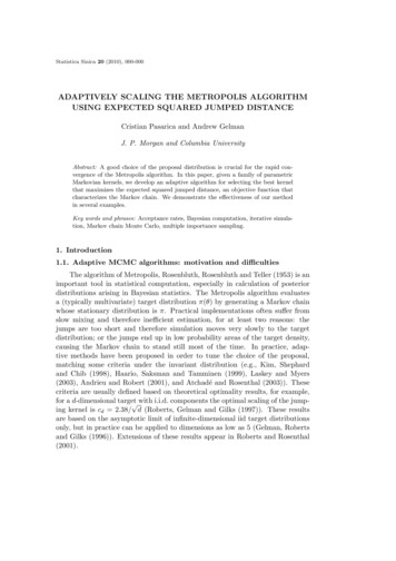
Monte-Carlo integrationMarkov chains and the Metropolis algorithmIsing modelConclusionSimulations of 2D Ising modelWe use the Ising model to demonstrate thestudies of phase transitions.The Ising model considers the interaction ofelementary objects called spins which arelocated at sites in a simple, 2-dimensionallattice,Ĥ JNXi,j nn(i)Figure: Lattice spinmodel with nearestneighbor interaction. Thered site interacts onlywith the 4 adjacentyellow sites.Ŝi Ŝj µ0 BNXi 1Magnetic ordering:J 0: lowest energy state isferromagnetic,J 0: lowest energy state isantiferromagnetic.Ŝi .
Monte-Carlo integrationMarkov chains and the Metropolis algorithmIsing modelConclusionEquibrium propertiesMean energyHeat capacityMean magnetizationLinear magnetic susceptibilityhE i Tr Ĥ ρ̂,” hE i1 “ 22hEi hEi, TkB T 2 * N X hMi Si , i 1”“1χ hM 2 i hMi2 ,kB TC where hMi and hM 2 i are evaluated at zero magnetic field (B 0).
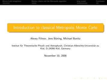
Monte-Carlo integrationMarkov chains and the Metropolis algorithmIsing modelMagnetization in 2D Ising model (J 0, L2 642 )Magnetization in 2D Ising model: L x L 64x64T 2.0Conclusion
Monte-Carlo integrationMarkov chains and the Metropolis algorithmIsing modelMagnetization in 2D Ising model (J 0, L2 642 )Magnetization in 2D Ising model: L x L 64x64T 2.30Conclusion
Monte-Carlo integrationMarkov chains and the Metropolis algorithmIsing modelMagnetization in 2D Ising model (J 0, L2 642 )Magnetization in 2D Ising model: L x L 64x64T 2.55Conclusion
Monte-Carlo integrationMarkov chains and the Metropolis algorithmIsing modelMagnetization in 2D Ising model (J 0, L2 642 )Magnetization in 2D Ising model: L x L 64x64T 3.90Conclusion
Monte-Carlo integrationMarkov chains and the Metropolis algorithmIsing modelConclusionStraightforward implementationIn each step we propose to flip a single spin, Si Si , and use the originalMetropolis algorithm to accept or reject.Phase-odering kinetics if we start from completely disordered state.T Tc Equilibration will be fast.T Tc Initial configuration is far from typical equilibrium state. Parallelspins form domains of clusters. To minimize their surface energy, thedomains grow and straighten their surface.For T Tc it is improbable to switch from one magnetization to the other, sinceacceptance probability to flip a single spin in a domain is low e 4J σ , σ 2.We need to work out more efficient algorithm.
Monte-Carlo integrationMarkov chains and the Metropolis algorithmIsing modelSimulations in critical regionAutocorrelation function near criticaltemperature Tc :A(i) A0 exp ( i/t0 ) i “Critical slowing down”t0 τO,int Lzz – dynamical critical exponent of thealgorithm. moreFor the original single spin-flip alrogithm z 2 in 2D.L 103 τO,int 105 . . . 106Conclusion
Monte-Carlo integrationMarkov chains and the Metropolis algorithmIsing modelConclusionClassical cluster algorithmsOriginal idea by Swendsen and Wang and later slightly modified by Niedermayerand Wolf. more1Look at all n.n. of spin σI and if theypoint in the same direction include themin the cluster C with the probability Padd .2For each new spin added to C repeat thesame procedure.3Continue until the list of n.n is empty.4Flip all spins in C simultaneously withprobability A.
Monte-Carlo integrationMarkov chains and the Metropolis algorithmIsing modelSpin-spin correlation.Spin spin correlation function.Correlation length2 1 T , L T T c L /2c r 〈 s i si r 〉 〈 s i 〉 〈 si r 〉 /〈 si 〉c r e r/ T T 2.0T 2.30 T T 2.55Conclusion
Monte-Carlo integrationMarkov chains and the Metropolis algorithmIsing modelL dependence: Magnet., suscep., energy, spec. heatSystem size L dependence:magnetization susceptibilityenergy specific heat 7 / 4 T T T c L T T c1/8m T T c T L T T cm T 0C L ,T c C 0 ln LConclusion
Monte-Carlo integrationMarkov chains and the Metropolis algorithmIsing modelFinite size scaling and critical properties.Finite size scaling and critical properties 1 T , L T T c L / 2T c L T c L T c L a L 1Numerical estimationfor critical temperature: k T estc L / J 2.2719 0.008Exact value: k T c L / J 2/ ln 1 2 2.26918Conclusion
Monte-Carlo integrationMarkov chains and the Metropolis algorithmIsing modelConclusionWhen/Why should one use classical Monte Carlo?Advantages1Easy to implement.2Easy to run a fast code.3Easy to access equilibrium properties.Disadvantages1Non-equilibrium properties are not accessible ( Dynamic Monte Carlo).2No real-time dynamics information ( Kinetic Monte Carlo).Requirements1Good pseudo-random-number generator, e.g. Mersenne Twister (period219937 1).2Efficient ergodic sampling.3Accurate estimations of autocorrelation times, statistical error, etc.
Monte-Carlo integrationMarkov chains and the Metropolis algorithmIsing modelFinThanks for your attention!Next lecture: Monte Carlo algorithms for quantum systemsConclusion
AppendixMarkov chain (Markov process)backThe Markov chain is the probabilistic analogue of a trajectory generated by theequations of motion in the classical molecular dynamics.We specify transition probabilities υ(Ri , Ri 1 ) from one state Ri to a newstate Ri 1 (different degrees of freedom in the system).We put restrictions on υ(Ri , Ri 1 ):1234The conservation law (the totalPprobability that the system willreach some state Ri is unity): Ri 1 υ(Ri , Ri 1 ) 1, for all Ri .TheP distribution of Ri converges to the unique equilibrium state:Ri p(Ri )υ(Ri , Ri 1 ) p(Ri 1 ).Ergodicity: The transition is ergodic, i.e. one can move from anystate to any other state in a finite number of steps with a nonzeroprobability.All transition probabilities are non-negative: υ(Ri , Ri 1 ) 0, forall Ri .In thermodynamic equilibrium, dp(R)/dt 0, we impose an additionalcondition – the detailed balancep(Ri )υ(Ri , Ri 1 ) p(Ri 1 )υ(Ri 1 , Ri ),
AppendixErgodicityIn simulations of classical systems we need to consider only configurationintegral„«3N/2 ZhiN12πmkB Tclass β ĤQNVT Tr e drN e βV (r )N!h2The average over all possible microstates {rN } of a system is called ensembleaverage.This can differ from real experiment: we perform a series of measurementsduring a certain time interval and then determine average of thesemeasurements.Example: Average particle density at spatial point r1ρ̄(r) limt tZt0dt 0 ρ(r, t 0 ; rN (0), pN (0))
AppendixErgodicitySystem is ergodic: the time average does not depend on the initialconditions. We can perform additional average over many different initial conditions(rN (0), pN (0))Zt11 Xρ̄(r) limt dt 0 ρ(r, t 0 ; rN (0), pN (0))N0tN00N0 is a number of initial conditions: same NVT , different rN (0), pN (0).ρ̄(r) hρ(r)iNVEtime average ensemble averageNonergodic systems: glasses, metastable states, etc.
AppendixAutocorrelationsbackAlgorithm efficiency can be characterized by the integrated autocorrelation timeτint and autocorrelation function A(i):τO,int 1/2 KXi 1A(i) (1 i/K ),A(i) 1hO1 O1 i i hO1 ihO1 i i.σO2Temporal correlations of measurements enhance the statistical error:srq22pσO2 ihOi hOiii2τO,int , Keff K /2τO,int . Ō σŌ2 KKeff
AppendixDetailed balance for cluster algorithmsbackDetailed balance equation(1 Padd )Kν Pacc (ν ν 0 )e βEν (1 Padd )Kν 0 Pacc (ν 0 ν)e βEν 0Probability to flip all spins in C :A Pacc (ν ν 0 ) (1 Padd )Kν 0 Kν e 2J β (Kν 0 Kν )Pacc (ν 0 ν)If we choose Padd 1 e 2 J β A 1, i.e every update is accepted.T Tc : Padd 0, only few spins in C (efficiency is similar to the singlespin-flip)T Tc : Padd 1, we flip large spin domains per one step.Wolf algorithm reduces the dynamical critical exponent to z 0.25. Enormousefficiency gain over the single spin-flip!
Monte-Carlo integration Markov chains and the Metropolis algorithm Ising model Conclusion Introduction to classical Metropolis Monte Carlo Alexey Filinov, Jens B oning, Michael Bonitz Institut fur Theoretische Physik und Astrophysik, Christian-Albrechts-Universit at zu Kiel, D-24098 Kiel, Germany November 10, 2008