Transcription
Munich Personal RePEc ArchiveHow to Create a Monte Carlo SimulationStudy using R: with Applications onEconometric ModelsAbonazel, Mohamed R.30 December 2015Online at https://mpra.ub.uni-muenchen.de/68708/MPRA Paper No. 68708, posted 09 Jan 2016 20:08 UTC
WorkshopHow to Create a Monte Carlo SimulationStudy using R: with Applications onEconometric ModelsDr. Mohamed Reda AbonazelDepartment of Applied Statistics and EconometricsInstitute of Statistical Studies and ResearchCairo Universitymabonazel@hotmail.com2015
SummaryIn this workshop, we provide the main steps formaking the Monte Carlo simulation study using Rlanguage. A Monte Carlo simulation is very commonused in many statistical and econometric studies bymany researchers. We will extend these researchers withthe basic information about how to create their R-codesin an easy way. Moreover, this workshop provides someempirical examples in econometrics as applications.Finally, the simple guide for creating any simulation Rcode has been produced.Page 1 of 29Mohamed R. Abonazel: A Monte Carlo Simulation Study using R
Contents of the workshop1. Introduction to Monte Carlo Simulation.2. The history of Monte Carlo methods.3. The advantages of Monte Carlo methods.4. The methodology of Monte Carlo methods inliteratures.5. The full steps to create a Monte Carlo simulationstudy (the proposed technic).6. The Application: Multiple linear regression modelwith autocorrelation problem.7. General notes on simulation using R.Page 2 of 29Mohamed R. Abonazel: A Monte Carlo Simulation Study using R
1. Introduction to Monte Carlo Simulation Gentle (2003) defined the Monte Carlo methods, ingeneral, are the experiments composed of randomnumbers to evaluate mathematical expressions To apply the Monte Carol method, the analystconstructs a mathematical model that simulates a realsystem. A large number of random sampling of the model isapplied yielding a large number of random samples ofoutput results from the model. For each sample, random data are generated on eachinput variable; computations are run through the modelyielding random outcomes on each output variable. Since each input is random, the outcomes are random.Page 3 of 29Mohamed R. Abonazel: A Monte Carlo Simulation Study using R
2. The history of Monte Carlo methods The Monte Carlo method proved to be successful andwas an important instrument in the ManhattanProject. After the World War II, during the 1940s, themethod was continually in use and became aprominent tool in the development of the hydrogenbomb. The Rand Corporation and the U.S. Air Force weretwo of the top organizations that were funding andcirculating information on the use of the Monte Carlomethod. Soon, applications started popping up in all sorts ofsituations in business, engineering, science andfinance.Page 4 of 29Mohamed R. Abonazel: A Monte Carlo Simulation Study using R
3. The advantages of Monte Carlo methodsWe can summarize the public advantages (goals) ofMonte Carlo methods in the following points: Make inferences when weak statistical theory existsfor an estimator Test null hypotheses under a variety of conditions Evaluate the quality of an inference method Evaluate the robustness of parametric inference toassumption violations Compare estimator’s propertiesPage 5 of 29Mohamed R. Abonazel: A Monte Carlo Simulation Study using R
4. The methodology of Monte Carlo methods inliteraturesMooney (1997) presents five steps to make a MonteCarlo simulation study:Step1: Specify the pseudo-population in symbolicterms in such a way that it can be used to generatesamples by writing a code to generate data in aspecific method.Step2: Sample from the pseudo-population in ways thatshow the topic of interestStep3: Calculate θ in a pseudo-sample and store it in avectorPage 6 of 29Mohamed R. Abonazel: A Monte Carlo Simulation Study using R
Step4: Repeat steps 2 and 3 t-times where t is thenumber of trialsStep5: Construct a relative frequency distribution ofresulting values which is a Monte Carlo estimateof the sampling distribution of under theconditions specified by the pseudo-population andthe sampling procedures For more details about Monte Carlo methods, youcan review the following references: Thomopoulos(2012), Gentle et al. (2012), and Robert and Casella(2013).Page 7 of 29Mohamed R. Abonazel: A Monte Carlo Simulation Study using R
5. The proposed technic: The full steps to createa Monte Carlo simulation study In this section, we proved the completed algorithm ofMonte Carlo simulation study. We explain our algorithm through an application inregression framework, especially; we will use theMonte Carlo technic to prove that OLS estimators ofGLR model are BLUEs.That algorithm contents five main stages as follows:Stage one: Planning for the studyIn this stage, we should put the plan to oursimulation study; the plane contains many importantsubjects:Page 8 of 29Mohamed R. Abonazel: A Monte Carlo Simulation Study using R
Satisfy our goals of the study (prove that OLSestimators of GLR model are BLUEs) Studying and understanding the model that willuse in the study. (Studying theoretically frameworkof the GLR model)The GLR model is given as:(1)whereisdependent vector,isindependent variables matrix,isunknownparameters vector, and iserror term vector.Assumptions:A1: ( )A2:()is non-stochastic matrix and(Mohamed R. Abonazel: A Monte Carlo Simulation Study using R)Page 9 of 29
A3:( )is full column rank matrix, i.e.,The OLS estimator of̂is given as:().(2) Satisfy the simulation controls (sample size (n),number of the independent variables (),standard deviation of the error term ( ),theoretical assumptions of the GLR model (A1 toA3 above), and so on ) Satisfy the criteria that will calculate in thesimulation study (Bias and variance of OLSestimators, that are given as):(̂)̂(̂)()(3)Page 10 of 29Mohamed R. Abonazel: A Monte Carlo Simulation Study using R
Note that these criteria are given in econometricliterature, but if they are not given theoretically, wecan calculate them by simulation. As an example,see Abonazel (2014a), Youssef et al. (2014), andYoussef and Abonazel (2015).Stage two: Building the modelWe can build our model by generate all thesimulation controls. In this stage, we must follow thefollowing steps by order:Step 1: Suppose any values as true values of theparameters vector .Step 2: Choose the sample size n.Step 3: generate the random generate the of the errorvector u under the model assumptions.Page 11 of 29Mohamed R. Abonazel: A Monte Carlo Simulation Study using R
Step 4: Generate the fixed values of the independentvariables matrix X under A2 and A3.Step 5: Generate the values of dependent variable byusing the regression equation, since we well know.Stage three: The treatment Once we obtain Y vector plus X matrix, thus wesuccesses to build our model under the satisfiedassumptions. Now we ready to make the treatment has beensatisfied in planning stage. The treatment is exactlycorrelated with the goals of our study. In ourexample, the treatment is the estimation of theregression parameters by using OLS method andthen proves that OLS estimators are BLUEs.Page 12 of 29Mohamed R. Abonazel: A Monte Carlo Simulation Study using R
We can summarize the treatment stage in thefollowing steps:Step 1: Regress Y on X by using the OLS formula inequation (2), then obtain the OLS estimations ̂ .Step 2: Calculate the criteria that have been satisfiedplanning stage. Then we calculate( ̂ ) and( ̂ ) by using equation (3).Stage four: The Replications Once we end the treatment stage, we obtain thevalues of biases and variances for only oneexperiment (one sample), then we cannotdependence with these values. To solve that, weshould make the following:Page 13 of 29Mohamed R. Abonazel: A Monte Carlo Simulation Study using R
Step 1: Repeat this experiment (L-1) times, each timeusing the same values of the parameters andindependent variables, if n and k are not changed.Of course, the u values will vary from experimentto experiment even though n and k are notchanged. Therefore, in all we have L experiments,thus generating L values each of biases andvariances.1Step 2: Take the averages of these L estimates and callthem Monte Carlo estimates:(̂) ̂(4)1In practice, many such experiments are conducted sometimes 1000 to2000. See Gujarati (2003).Page 14 of 29Mohamed R. Abonazel: A Monte Carlo Simulation Study using R
(̂) (̂)(5)Stage five: Evaluating and presenting the results After ending the treatment stage, we must checkand evaluate the simulation result before put ordiscuss (display) it in our paper (research). The evaluation process aims to answer an importantquestion: Are the results consistent with thetheoretical framework or not? If the answer is yes, thus these results can be reliedupon. But in a case of the results are inconsistent with thetheoretical framework, we must review and/orPage 15 of 29Mohamed R. Abonazel: A Monte Carlo Simulation Study using R
repeat the four stages with more accuracy to catchthe mistake and correct it. The reviewing process contains two branches. First,review the theoretical framework of the modelfrom different books or papers. Second, reviewyour software program, there may beprogrammatic mistakes. After this evaluation, we can repeat calculate thesimulation criteria again in different situations(apply the simulation factors), this step is veryimportant because it gives us general image andmore analysis of the studied model.Page 16 of 29Mohamed R. Abonazel: A Monte Carlo Simulation Study using R
In the end, the results should be consistent with thetheoretical framework. And then, we should displaythese results using a properly method. There are two main methods, to provide anysimulation results, are tables and graphs. Theresearcher chooses between tables and graphs basedon the contribution made by each method. For more details about the simulation technics thatused in econometrics, you can review the followingreferences: Craft (2003) and Barreto and Howland(2005).Page 17 of 29Mohamed R. Abonazel: A Monte Carlo Simulation Study using R
6. The Application: Multiple linear regressionmodel with autocorrelation problemIn this application, we apply the abovealgorithm of Monte Carlo technic to comperebetween OLS and GLS estimators in multiple linearregression model when the errors are correlated withfirst-order autoregressive (AR(1)). In each stage, weproved R-code to create it. In this workshop, wesuppose that the reader is familiar with Rprograming basics. If you are not satisfied that, youcan review the following references: Robert andCasella (2009), Crawley (2012), and Abonazel(2014b).Stage one: Planning for the studyNow we apply the first stage, so we satisfy fourfactors as follows:1. Satisfy our goal of the study: The goal iscompere between the performance of OLS andGLS estimators in multiple linear regressionmodel when the errors are correlated with firstorder.Page 18 of 29Mohamed R. Abonazel: A Monte Carlo Simulation Study using R
2. Studying theoretically framework of the model:this model is given in equation (1), where A2 andA3 are still valid, but A1 will be replaced to thefollowing assumption:A4:(whereand ()The OLS and GLS estimators ofA4 are:̂(where();)̂(()),.under A2 to))(Since the elements of are usually unknowns,we develop a feasible Aitken estimator of basedon consistent estimators of it:̂ ̂ ̂̂where ̂ are the residuals from apply OLS, andPage 19 of 29Mohamed R. Abonazel: A Monte Carlo Simulation Study using R
where ̂.̂ ̂ ̂ , and̂̂̂̂̂3. Satisfy the simulation controls: Table 1 displaysthe full details about the simulation factors.Table (1): The simulation factorsNo. Simulation Factor1The true values of theparameters ( )2Sample size ( )3The AR(1) coefficient ( )Levels(where 2 ) 5, 15, 30, and500.50and0.904The variance of the error term( )1 and 54. Satisfy the study criteria: The criteria here arethe bias and variance of OLS and GLS estimatorsthat are given in this model as:Page 20 of 29Mohamed R. Abonazel: A Monte Carlo Simulation Study using R
(̂)(̂̂)(̂())((̂Stage two: Building the model)()̂)We can build our model by generate all thesimulation controls (factors) as given in table (1). TheR-code is:#---- Stage two: Building the model#---- Step 1: Suppose the true values of the parameters vector β :True.Beta - c(1,1)#---- Step 2: Choose the sample size n:n 5#---- Step 3: generate the random generate the of the error vector uunder A1:sigma.epsilon sqrt(1)rho 0.50epsilon rnorm(n,0, sigma.epsilon)u c(0)u[1] epsilon[1]/((1-(rho) 2) 0.5)for(i in 2:n) u[i] rho*u[i-1] epsilon[i]#---- Step 4: Generate the fixed values of the independent variablesmatrix X under A2 and A3:X cbind(1,runif(n,-1,1))#---- Step 5: Generate the values of dependent variable Y :Y X%*%True.Beta uPage 21 of 29Mohamed R. Abonazel: A Monte Carlo Simulation Study using R
Stage three: The treatment#---- Stage three: The treatment (by cerate estimation function):estimation -function(Y Y,X X){#---- Step 1: calculate OLS and GLS estimators##1 ---- OLS estimator:Beta.hat.ols solve(t(X) %*% X) %*% t(X) %*% Y## 2 ----GLS estimator:rho.hat (t(u[-n] )%*% u[-1])/sum(u[-1] 2)dim(rho.hat) NULLif(rho.hat 1) rho.hat 0.99; if(rho.hat 0) rho.hat 0.005#-----------------epsilon.hat NAepsilon.hat[1] u[1]*(1 - (rho.hat) 2) 0.5epsilon.hat[2:n] u[-1] rho.hat * u[-n]sigma2.epsilon.hat sum(epsilon.hat 2)/(n-2)dim(sigma2.epsilon.hat) NULL#-----------------v - matrix(NA,nrow n,ncol n)for (i in 1:n) for (j in 1:n) v[i,j] (rho.hat) abs(i - j)omega - (sigma2.epsilon.hat / (1 - (rho.hat) 2)) * vBeta.hat.gls solve(t(X) %*% solve(omega) %*% X) %*% (t(X) %*%solve(omega) %*% Y)#---- Step 2: Calculate the Simulation criteria (bias and variance)bias.ols Beta.hat.ols - True.Betabias.gls Beta.hat.gls - True.Betavar.Beta.hat.gls diag(solve(t(X) %*% solve(omega) %*% X))var.Beta.hat.ols diag (solve(t(X) %*% X) %*% t(X) %*% omega%*% X %*% solve(t(X) %*% X))BV cbind(bias.ols, bias.gls, var.Beta.hat.ols, var.Beta.hat.gls)rownames (BV) c("Beta0","Beta1")colnames(BV) c("Bias OLS","Bias GLS", "Var OLS","Var GLS")return (BV) }Page 22 of 29Mohamed R. Abonazel: A Monte Carlo Simulation Study using R
Stage four: The ReplicationsOnce we end the treatment stage, we obtain thevalues of biases and variances for only oneexperiment (one sample). Therefore, we Repeat thisexperiment (L-1) times, and then take the averagesof these L estimates as follows:#---- Stage four: The ReplicationsL 5000Sim.results matrix (0,nrow 2,ncol 4)for (l in 1:L) {epsilon rnorm(n,0, sigma.epsilon)u c(0)u[1] epsilon[1]/((1-(rho) 2) 0.5)for(i in 2:n) u[i] rho*u[i-1] epsilon[i]Y X%*%True.Beta uresults.matrix estimation (Y Y,X X)Sim.results Sim.results results.matrix}average Sim.results /laveragewrite.table(average, "clipboard", sep "\t", col.names NA )Page 23 of 29Mohamed R. Abonazel: A Monte Carlo Simulation Study using R
Stage five: Evaluating and presenting the resultsAfter ending the treatment stage, we must checkand evaluate the simulation result. The evaluationprocess aims to answer an important question: Arethe results consistent with the theoretical frameworkor not?Table (2): Simulation results when 5,( ),1, and0.50Bias OLS Bias GLSVar OLSVar GLSBeta0 -0.00063 -0.00608 48.84283 47.66144Beta1 0.029276 0.04247616.0963 10.58763Note that: Bias and variance for GLS estimates areless than the bias and variance of OLS estimates, thisresult is consistent with the theoretical framework, thenwe can rely on these results.After this evaluation, we can repeat calculate thesimulation criteria again in different situations. In otherwords, we calculate the values of biases and variancesunder different simulation factors as given in table (1).And then, we should display these results using aproperly method. Here we will use the tables.Page 24 of 29Mohamed R. Abonazel: A Monte Carlo Simulation Study using R
#---- Complete Program after definition our function (estimation)###------------Not Fixed------------n c(5,15,30,50)rho c(0.50, 0.90)sigma.epsilon sqrt(c(1,5))#----------------Fixed ---------------True.Beta - c(1,1)L 1000Sim.results matrix (0,nrow 2,ncol 4)Final.table array(NA,c(16,8))colnames(Final.table) c("n 5","n 5","n 15","n 15","n 30","n 30","n 50","n 50")#-----------------------------------------ro 0for (rhoi in 1:2) {se 0for (sigma in 1:2) {sz 0for (ni in 1:4) {X cbind(1,runif(n[ni],-1,1))for (l in 1:L) {epsilon rnorm(n[ni],0, sigma.epsilon[sigma])u c(0)u[1] epsilon[1] / ((1 - (rho[rhoi]) 2) 0.5)for (i in 2:n[ni])u[i] rho[rhoi] * u[i - 1] epsilon[i]Y X %*% True.Beta uresults.matrix estimation (Y Y,X X)Sim.results Sim.results results.matrix} ## for laverage Sim.results / lFinal.table[(ro se 1):(ro se 4),(sz 1):(sz 2)] - t(average)sz sz 2 }##for nise se 4 } ## for sigmaro ro 8} ## for rhoiFinal.tablewrite.table(Final.table, "clipboard", sep "\t", col.names NA )Page 25 of 29Mohamed R. Abonazel: A Monte Carlo Simulation Study using R
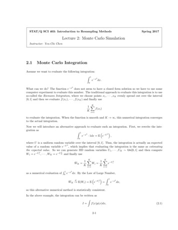
Table (3): The results of the Monte Carlo study when thereplications 10005Bias OLSBias GLSVar OLSVar GLSBias OLSBias GLSVar OLSVar GLSBias OLSBias GLSVar OLSVar 0.1000.0640.098995.25729.104 1288.57638.887 1478.91941.730 1554.47443.076988.12522.141 1272.72324.514 1453.56825.450 1522.19825.9640.313Bias OLS0.327Bias GLSVar OLS 5151.000Var GLS 2800.2080.2640.1810.2720.173316.166 7051.481339.658 8519.216 352.380 8895.343 390.531222.181 6950.816236.186 8366.166 241.435 8705.211 244.697 If you are want to display the simulation results in graphs,see, e.g., Abonazel (2009, Appendix B) for 2D graphs,while for 3D graphs, see, e.g., Abonazel (2014a, AppendixB) and Youssef and Abonazel (2015).Page 26 of 29Mohamed R. Abonazel: A Monte Carlo Simulation Study using R
In the previous example, we have studied the estimationproperties of single-equation regression model. Howeverthere are studies are used the Monte Carlo simulationtechnics for multi-equation regression models (such aspanel data models), see, e.g., Youssef and Abonazel(2009) and Mousa et al. (2011).7. General notes on simulation using R R is considered one of the fastest packages forsimulation. If the simulation time took too long or you want to endthe processing, you can press the red icon "STOP" inthe tool menu anytime. Two way to reduce the bias (bias mean ofexperiments – true value):o By increase the sample size.o By increase the number of iterations but it willnot be as effective. In loops, we can create nested loops (a loop inside aloop) very easily. For example: loop for i and loop for jinside it, i.e. for i (for j)Page 27 of 29Mohamed R. Abonazel: A Monte Carlo Simulation Study using R
In iterations, it is highly recommended to omit thefirst 50 iterations from the calculations (such as bias orvariances values)References1. Abonazel, M. R. (2009). Some properties of random coefficientsregression estimators. MSc thesis. Institute of Statistical Studiesand Research. Cairo University.2. Abonazel, M. R. (2014a). Some estimation methods for dynamicpanel data models. PhD thesis. Institute of Statistical Studies andResearch. Cairo University.3. Abonazel, M. R. (2014b). Statistical analysis using R, AnnualConference on Statistics, Computer Sciences and OperationsResearch, Vol. 49. Institute of Statistical Studies and research,Cairo University. DOI: 10.13140/2.1.1427.2326.4. Barreto, H., Howland, F. (2005). Introductory econometrics: usingMonte Carlo simulation with Microsoft excel. CambridgeUniversity Press.5. Craft, R. K. (2003). Using spreadsheets to conduct Monte Carloexperiments for teaching introductory econometrics. SouthernEconomic Journal, 726-735.6. Crawley, M. J. (2012). The R book. John Wiley & Sons.7. Gentle, J. E. (2003). Random number generation and Monte Carlomethods. Springer Science & Business Media.8. Gujarati, D. N. (2003) Basic econometrics. 4th ed. McGraw-HillEducation.9. Gentle, J. E., Härdle, W. K., Mori, Y. (2012). Handbook ofcomputational statistics: concepts and methods. Springer Science& Business Media.Page 28 of 29Mohamed R. Abonazel: A Monte Carlo Simulation Study using R
10.Mooney, C. Z. (1997). Monte Carlo simulation. Sage UniversityPaper Series on Quantitative Applications in the Social Sciences,series no. 07-116. Thousand Oaks, CA: Sage.11.Mousa, A., Youssef, A. H., Abonazel, M. R. (2011). A MonteCarlo study for Swamy’s estimate of random coefficient panel datamodel. Working paper, No. 49768. University Library of Munich,Germany.12.Robert, C., Casella, G. (2009). Introducing Monte Carlo Methodswith R. Springer Science & Business Media.13.Robert, C., Casella, G. (2013). Monte Carlo statistical methods.Springer Science & Business Media.14.Thomopoulos, N. T. (2012). Essentials of Monte Carlo Simulation:Statistical Methods for Building Simulation Models. SpringerScience & Business Media.15.Youssef, A. H., Abonazel, M. R. (2009). A comparative study forestimation parameters in panel data model. Working paper, No.49713. University Library of Munich, Germany.16.Youssef, A. H., Abonazel, M. R. (2015). Alternative GMMestimators for first-order autoregressive panel model: an improvingefficiency approach. Communications in Statistics-Simulation andComputation (in press). DOI: 10.1080/03610918.2015.1073307.17.Youssef, A. H., El-sheikh, A. A., Abonazel, M. R. (2014). NewGMM estimators for dynamic panel data models. InternationalJournal of Innovative Research in Science, Engineering andTechnology 3:16414–16425.Page 29 of 29Mohamed R. Abonazel: A Monte Carlo Simulation Study using R
Mohamed R. Abonazel: A Monte Carlo Simulation Study using R Contents of the workshop 1. Introduction to Monte Carlo Simulation. 2. The history of Monte Carlo methods. 3. The advantages of Monte Carlo methods. 4. The methodology of Monte Carlo methods in literatures. 5. The full steps to create a Monte Carlo simulation study (the proposed .