Transcription
A Practical Guide toModeling FinancialRisk with MATLAB
A Practical Guide to ModelingFinancial Risk with MATLAB1. Introduction to Risk Management2. Credit Risk Modeling3. Market Risk Modeling4. Operational Risk Modeling
Chapter 1:Introduction to Risk Management
What is risk management?Risk management is a process that aims to efficiently mitigate and control the risk in an organization. The life cycleof risk management consists of risk identification, risk assessment, risk control, and risk monitoring. In addition,risk professionals use various mathematical models and statistical methods (e.g., linear regression, Monte Carlosimulation, and copulas) to quantify the potential loss that could arise from each type of gRiskControlThe risk management cycle.A Practical Guide to Modeling Financial Risk with MATLAB4
What is the origin of risk?The major role of financial institutions in the economy is to be amiddleman in credit card, mortgage, bond, stock, currency, mutual fund,and other financial transactions. By participating in these transactions,financial institutions expose themselves to a lot of uncertainty, such asprice movements, the chance that a borrower may not repay a loan, orhuman error from the staff.Risk regulation usually evolves rapidly in the aftermath of financialcrisis. For instance, in 2007–2008, a subprime mortgage crisis not onlyled to a global banking crisis, but also played significant role in thedevelopment of the Dodd-Frank Act, Basel III, IFRS 9, and CECL.“Risk comes from not knowing what you’re doing.”— Warren Buffett“The biggest risk is not taking any risk In a worldthat’s changing really quickly, the only strategy that isguaranteed to fail is not taking risks.”— Mark ZuckerbergProducts in intermediary services of financial institutions.A Practical Guide to Modeling Financial Risk with MATLAB5
What types of risk do financial institutions face?Large financial institutions have sophisticated holding structures withmany financial subsidiaries. In addition, these financial institutions mayoperate under a universal banking model to provide a variety of servicesand products to clients. As a result, these financial institutions face manytypes of risks. The three most common risk types for an organization are: Credit risk: the potential for a loss when a borrower cannot makepayments to a lender Market risk: the potential for a loss resulting from the movement ofasset prices Operational risk: the potential for a loss arising from people,processes, systems, or external events that influence a businessfunctionHowever, there are more specific types of risk that require the attentionof risk professionals, such as liquidity risk, capital risk, business risk,reputational risk, systemic risk, model risk, concentration risk, legal risk,moral hazard, and financial crime.Specialized financial institutions like central banks also face manyof these risks. Even though the best-known role for central banks is aregulator, they also act as liquidity providers and lenders of last resort.These two roles alone require central banks to take huge risk exposure.The main differences are that risk mitigation tools for central banksinclude macroeconomic policy and regulatory interventions.Types of risk faced by financial institutions.A Practical Guide to Modeling Financial Risk with MATLAB6
How do you quantify risk?There are two major approaches for riskquantification: qualitative and quantitativeapproaches. Qualitative approaches, suchas assessing a company’s overall strategy,are subjective in nature and managed aspart of the business decision-making process.Quantitative risk assessment involves definingthe probability of occurrence and potentialimpact of each type of risk important tothe organization’s business. Quantitativeassessment commonly uses statistical models,Monte Carlo simulations, time series models,optimization, machine learning, and othercomputational approaches.Techniques and issues concerning risk quantification (Word cloud generated using Text Analytics Toolbox ).A Practical Guide to Modeling Financial Risk with MATLAB7
Stress TestingStress testing is a form of scenario analysis used to gauge the impactof extreme scenarios (often called stress scenarios) on the financialinstitutions or investment portfolios. In the past decade, the importanceof stress testing has escalated because regulators around the worldadopted it as a tool to evaluate the strength of financial institutions undertheir supervision. For regulatory-based stress testing, regulators wouldpredefine a set of stress scenarios, where one scenario consists of manyvariables. Variables for stress testing usually cover macroeconomicvariables, equity prices, equity market volatility, real estate prices, andinterest rates.Learn how to use MATLAB for: Macroeconomic stress testing Consumer credit stress testing Contagion risk analysis using graph theory and hiddenMarkov models Incorporating stress scenarios into a forecasting model ofcorporate default ratesGiven the importance of stress testing and the complexity of financialinstruments held by financial institutions, risk managers need to have aplatform they can use to easily develop and deploy their risk models.Stress testing based on macroeconomic variables.A Practical Guide to Modeling Financial Risk with MATLAB8
Real-World ExamplesPractically speaking, risk management systems require modifications andcustomizations over time. Risk managers usually need to adjust their riskmanagement models to conform to new regulations or to address newtypes of risk factors.PZU Group developed a complete production-ready market risk solutionto comply with the Solvency II Directive. Such solutions could highlyaccelerate development time and computational time.Read the story: PZU Group Develops Market Risk Modelfor Solvency II CompliancePlot showing how minimizing the differences between real and expectedprobability densities helps PZU identify the risk-neutral density function.A Practical Guide to Modeling Financial Risk with MATLAB9
Learn MoreReady for a deeper dive? Explore these resources to learn more about riskmanagement methods, examples, and tools.WatchReadMunich Re Trading Creates a Risk AnalyticsPlatform with MATLAB: Demonstration (3:32)7 Chief Risk Officer Priorities for 2017Reforming Risk Management. Again?Use of MATLAB for Solvency II Capital Modelling:The Prudential Risk Scenario Generator (22:44)Can we fix Risk Management? Yes, we can.MATLAB Production Server for FinancialApplications (38:28)ExploreLearn more about using MATLAB in differentregulatory frameworks:BASEL IIISolvency IIIFRS 9
Chapter 2:Credit Risk Modeling
What is the expected loss from credit risk?The most common measure of credit risk is expected loss, which is the average loss in value of the credit portfolioover a given time period or the lifetime of the credit instrument. Depending on the nature of credit instruments, twoalternative ways to estimate the expected loss are by looking at default events only and by looking at the loss invalue due to the changes in credit quality or credit rating.A Practical Guide to Modeling Financial Risk with MATLAB12
Expected Loss Based on Default RiskTypically, the expected loss (EL) of a loan portfolio (e.g., credit card,home and auto loans, personal lending) can be measured throughthree independent factors: probability of default (PD), loss given default(LGD), and exposure at default (EAD).Example:If the amount of the loan is 100 and the expected value of thecollateral in the next year is 75, then:LGD (100 – 75) / 100 25%EL PD LGD EADGiven there is a 5% chance that car owners will default onauto loan, then:EL 5% 25% 100 1.25ELPDLGDEADA Practical Guide to Modeling Financial Risk with MATLAB13
Expected Loss Based onChanges in Credit RatingEven though the default event has not occurred yet, the value of a creditportfolio may change with credit rating. Such scenarios are readilyapparent in the bond market. In this case, you can adjust the earlierformula of expected loss (EL) to make it more generic as follows:EL Reference Value – iPi ValueiPi is the transition probability that the instrument would migrate from itscurrent rating to rating i.Valuei is the dollar value of the instrument after migrating from the currentrating to rating i.Characteristics of default risk and market valueof credit instruments by rating.Reference value is the end-of-period value at the current rating in dollars.Rating at the endof the periodAAAAA*ABBBBBBCCCDefaultP (%)1.0090.005.501.701.100.400.200.10Value ( )102101999590858030 iPi Valuei 100.50*Current ratingGiven the reference value of 101, EL 101–100.50 0.50Calculation example of expected loss from credit migration.A Practical Guide to Modeling Financial Risk with MATLAB14
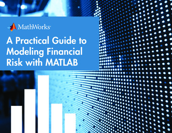
LessRiskLessRiskiskre RMoProbabilityofDefault(PD)iskre RMoEach credit risk model has its own parameters andassumptions depending on the definition of expected loss.One of the most practical steps in building a successful riskmodel is to get accurate assessment of risk parameters.For credit risk, the common risk parameters you need toestimate are:LessRiskEstimating Risk ParametersLossGivenDefault(LGD) Default-based model:o Credit migration matrix (also known as transitionprobability ult(EAD)iskre RMoProbabilityofDefault(PD)iskre RMoThe very common statistical technique for estimating riskparameters is regression (see fitglm or fitlm).LessRiskLessRisk Credit migration–based model:ProbabilityofDefault(PD)iskre RMoo Exposure at default (EAD)iskre RMoo Loss given default (LGD)LessRisko Probability of default (PD)A Practical Guide to Modeling Financial Risk with MATLAB15
Probability of DefaultThere are many ways to estimate probability of default (PD); your choicewill depend very much on assumptions and the availability of data.Commonly used models for estimating probability include: Structural models: The models use information from the company’scapital structure (e.g., asset, liability, and equity) to estimate PD. Oneof the most popular structural models is the Merton model. Reduced-form models: The PD can be estimated by extracting thedefault risk implied by market prices of credit instruments such asbond or credit default swap. Historical credit ratings migrations:Instead of directly model PD, youcan use credit history to estimate the transition probabilities that acredit instrument will migrate from one rating to another rating. Statistical approaches:A variety of statistical methods can be appliedto estimate the PD based on the given characteristics of the creditinstruments, for example:o Regression models (e.g., linear, logistic, probit, orCox-proporional hazards)The Binning Explorer app.o Machine Learning (e.g., tree bagger, random forest, ordiscriminant analysis)o Credit scoring modelsA Practical Guide to Modeling Financial Risk with MATLAB16
Credit Migration MatrixRATING HISTORYA credit migration matrix (also known as transitionprobability matrix) is a matrix in which each elementrepresents the probability of the credit instrumentsmigrating from one rating to another rating over a periodof time. The typical period for calculating credit migrationmatrix is one year. Two major ways to estimate the creditmigration matrix from historical credit rating migration dataare: Cohort estimation: The probabilities are estimated basedon a sequence of snapshots of credit ratings at regularlyspaced points in time. However, if there is more thanone change in credit rating between two snapshotdates, only the final rating will influence the estimates. Duration estimation (also known as hazard rateor intensity): The transition probabilities are estimatedbased on continuous time assumption using the fullcredit rating history, looking at the exact dates on whichthe credit rating migrations occur.Learn more: Estimating a Credit Migration MatrixUsing DIT MIGRATION 21.42944.289881.292712.7167D-.----.-.-. 100.0000A Practical Guide to Modeling Financial Risk with MATLAB17
Loss Given DefaultLoss given default (LGD) is a loss from the event of defaultthat is presented as a percentage of the exposure atdefault. Fundamentally, LGD is associated with manyfactors, including: Instrument-specific factors:o Loan collateralo Debt seniority Company-specific factors:o The company’s financial ratio Industry-specific factors Macro-level factorsIn fact, LGD can be defined as 1 – recovery rate.Regression models, scorecard models, and statisticallearning techniques, in general, can be used to predictrecovery rates. These models can include some of thefactors mentioned above (credit scores, financial ratios,macro variables) as predictors.Factors associated with loss given default (LGD).A Practical Guide to Modeling Financial Risk with MATLAB18
Exposure at DefaultExposure at default (EAD) is the amount of exposure at the time ofdefault. In fact, EAD is closely related to LGD because the multiplicationof these two parameters will give us the amount of loss at the time ofdefault. For this reason, EAD is also an instrument-specific parameter.The EAD’s distribution for fixed-income instruments is different from thatfor credit card loans.In addition to these indicators, the estimation of credit exposurefor derivative contracts (e.g., swaps or options) can be morecomputationally intensive because the credit exposure depends on themarket price of the underlying asset in the derivative contract too.Mathematically, EAD can be modeled as a function of current exposureand future potential exposure. The latter is more complicated because itusually deals with undrawn credit lines. For example, credit card loansand home equity lines of credit (HELOCs) are basic credit instruments inwhich a borrower can borrow up to a credit limit given by the lender. Inthe event of default, borrowers are likely to utilize more or max out theundrawn credit line.The table shows popular indicators for estimating EAD.IndicatorMathematical Definition in Relation to EADLoan Equivalent (LEQ)EAD Drawn Credit Line LEQ Undrawn Credit LineCredit Conversion Factor (CCF)EAD CCF Drawn Credit LineEAD Factor (EADF)EAD EADF Total Credit LineA Practical Guide to Modeling Financial Risk with MATLAB19
Credit Portfolio SimulationUnlike the analysis of credit risk on an individual basis you need tounderstand more about the aggregated credit risk, diversification,and concentration characteristics at the credit portfolio level. For thisreason, default correlations between counterparties and issuers play animportant role to help us understand the credit risk at a portfolio level.Two alternative frameworks for performing credit portfoliosimulation are: Under the assumption that the credit instruments have only two stages(default and non-default), you can simulate correlated variables anduse the copula method to map these variables to default and nondefault states to preserve the individual default probabilities. Given that the value of credit instruments may change with creditratings, you can simulate correlated variables, map these variables to acredit rating based on a credit migration matrix, and use the simulatedcredit rating scenarios to compute credit risk at a portfolio level.Both the default and credit migration simulations have an underlyingone-factor or multifactor model. The parameters of the factor model canbe estimated from market data, and these parameters imply a default orcredit migration correlation between counterparties that influences thecredit portfolio risk measures.Losses from credit portfolio simulation.Learn more: Credit Portfolio Simulation with MATLAB Credit Portfolio Simulation Based on Correlated Defaults Credit Portfolio Simulation Based on a Credit Migration MatrixA Practical Guide to Modeling Financial Risk with MATLAB20
Counterparty Credit Risk of Derivative ContractsCounterparty credit risk is the potential for a loss if thecounterparty to a derivative contract is unable to fulfillthe contractual obligations. Such counterparty risk canbe measured in terms of valuation adjustments. The mostpopular valuation adjustment is credit valuation adjustment(CVA), which is designed to capture the market value ofcounterparty risk to a derivative contract. Other valuationadjustments include funding valuation adjustment (FVA),debt valuation adjustment (DVA), collateral valuationadjustment (COLVA), and capital valuation adjustment(KVA). Unlike OTC derivatives, the counterparty risk oflisted derivatives is assumed to be zero because of theexistence of a central counterparty. However, the marketparticipants may be required to place initial margin andvariation margin. For this reason, only margin valuationadjustment is used to address these costs for listedderivatives. These valuation adjustments are collectivelyknown as X-value adjustment (XVA).Explore MATLAB examples on:DVAKVACVAX-ValueAdjustment (XVA)COLVAFVAX-value adjustment. Calculating counterparty risk and CVA Calculating wrong-way riskA Practical Guide to Modeling Financial Risk with MATLAB21
Calculating Regulatory Capital for Credit RiskFinancial institutions are obligated to maintain their capital level above a minimum requirement, which is calculated based on their risk exposure.Since credit risk was responsible for many of the greatest losses in the financial history, calculating of regulatory capital for credit risk is an essentialtask for financial institutions to help them perform efficient capital management, risk budgeting, and financial modeling.STANDARDIZED APPROACH (SA)Risk WeightCredit RiskCapital RequirementConstantExposureFOUNDATION INTERNAL-RATING BASED APPROACH (FIRB)Risk ModelCredit RiskCapital RequirementConstantEADPDLGDMADVANCED INTERNAL-RATING BASED APPROACH (AIRB)Risk ModelCredit RiskCapital RequirementConstantParameters estimated by financial institutionsEADPDLGDMEAD exposure at default, LGD loss given default,M effective maturity, Constant Risk-based multiplier defined by the regulatorSA and IRBs for calculating credit risk capital.A Practical Guide to Modeling Financial Risk with MATLAB22
Calculating Regulatory Capital for Credit RiskcontinuedPer the Basel Accords, two major approaches for calculating credit riskcapital are: Standardized approach (SA). Financial institutions can easily calculatecapital requirements using a simplified framework provided by theregulator. However, it usually produces higher capital requirementsthan the IRB approach. Internal-rating based approach (IRB). The IRB can be categorizedbased on the complexity level into foundation IRB (FIRB) andadvanced IRB (AIRB). Financial institutions need to estimate onlyprobability of default (PD) by themselves in FIRB, while they need toestimate more parameters in AIRB. To simplify the IRB framework andmake it scalable, the asymptotic single risk factor (ASRF) model wasintroduced as a tool for calculating regulatory capital for credit risk.Because it is more complex than SA, IRB is more expensive in termsof administration and supervision, but it is likely to achieve lowerregulatory capital requirements.Explore MATLAB examples on: Calculating regulatory capital with the ASRF model Modeling correlated defaults with copulasA Practical Guide to Modeling Financial Risk with MATLAB23
Real-World ExamplesSwiss Re, founded in 1863, based in Zurich, is the world’ssecond largest reinsurer and has a long history of using aninternal risk model to steer the company. The model defines itstarget capital, sets risk-based business volume limits, allocatescapital costs across various lines of business, determinesthe company’s solvency ratio for regulatory purposes (SwissSolvency Test, Solvency II), and more.For a decade, Swiss Re has used MATLAB to implement theInternal Capital Adequacy Model (ICAM), its internal risk model.Dynamic and increasingly complex internal and regulatoryrequirements create a challenging development environment, inwhich MATLAB proved to be the perfect development platformto quickly react to changing requirements. In 2017, Swiss Reconcluded a major project to overhaul its internal risk model, thekey goals being transparency, flexibility for future developments,speed, and precision of risk measures.Learn how Swiss Re develops and maintains its internalrisk model in MATLAB.A Practical Guide to Modeling Financial Risk with MATLAB24
Learn MoreReady for a deeper dive? Explore these resources to learn more aboutcredit risk modeling, examples, and tools.WatchCredit Risk Modeling with MATLAB (53:10)Financial Model Validation Using MATLAB (33:01)Credit Scorecard Modeling Using the Binning Explorer App (6:17)ReadBasel II Compliance and Risk Management Analysis: Calculating Economic CapitalModeling Corporate Credit RiskExploreRisk Management Toolbox Risk Management with MATLAB
Chapter 3:Market Risk Modeling
What is market risk?Market risk is the potential for a loss in thevalue of a portfolio due to the change inmarket prices. Commonly, market risk can begrouped by underlying assets or major factorsthat affect the pricing of financial instruments,for example, equity risk, commodity risk,foreign exchange risk, interest rate risk,and volatility risk. In addition, market riskis typically the largest exposure for buyside financial institutions, such as assetmanagement companies, hedge funds, andproprietary trading houses.A Practical Guide to Modeling Financial Risk with MATLAB27
Pricing of Financial InstrumentsTo measure market risk, it is essential to estimate the current value ofthe portfolio as well as the potential changes in value of all financialinstruments within it. In some cases, a market risk analyst may need tocalculate the theoretical prices of financial instruments when marketprices do not exist. For this reason, a lot of work in market risk analysisinvolves pricing and modeling financial instruments.In fact, the complexity of financial models varies greatly from onefinancial instrument to another. For example, European options can besimply priced by using a closed-form formula, whereas you may need toperform more complicated computation for exotic options. In addition,the model that works well in one market may not be able to producethe same result in another market. That is why market risk analystsoften need to customize the pricing models in many circumstances, forinstance, new products, changes in underlying assumptions, specificmarket practices, or constraints.Read more about pricing of these financial instruments: Equity derivatives Energy derivatives Credit derivatives Interest rate instrumentsA Practical Guide to Modeling Financial Risk with MATLAB28
Estimating Market Risk ParametersSeveral risk parameters are commonly used to estimate risk measures orprice financial instruments like interest rates, volatilities, and correlations.Depending on your objectives and the importance of each variable, youmight use a parameter estimate based on historical values, current value,implied value, or forecasted value as input in your financial models.Volatilities are among the most important risk parameters. For pricingpurposes, implied volatility values are important to determine pricesthat are consistent with the current market conditions. For risk analysis,you may prefer to forecast the volatility during the lifetime of the optioncontract using econometrics models (e.g., GARCH, EGARCH, or GJR).On the other hand, if you are dealing with interest rate derivatives,there are multiple interest rate models to choose from, and these modelsmay have different parameters. So, it is very important to determine theinterest rate model before estimating its model parameters (e.g., driftterm and volatility). Then you can perform simulation or forecast theinterest rates based on the estimated model parameters to price interestrate derivatives or to calculate risk measures. Popular interest modelsinclude: Heath-Jarrow-Morton Model Black-Derman-Toy (BDT) Model Black-Karasinski (BK) Model Hull-White (HW) Model Libor Market Model Diebold Li Model Nelson-Siegel Model Negative-rate models(e.g., Shifted SABR Modeland Shifted Black Model)Learn more: Calibration and Simulationof Interest Rate ModelsThe growing set of risk parameters.A Practical Guide to Modeling Financial Risk with MATLAB29
Monte Carlo SimulationAmong the mathematical techniques used in market risk modeling,Monte Carlo simulation is one of the most basic and most importantframeworks that are widely used behind the scene. You can use MonteCarlo simulation in a variety of risk applications, such as:Explore how to simulate: Analyzing worst-case scenarios and potential profit/loss Conditional mean and variance models Pricing and valuation of financial instruments Equity markets using geometric Brownian motion (GBM) Incorporating uncertainty factors into existing risk models Multidimensional stochastic differential equations (SDEs) Random numbers from the numerous distributions Term structure of interest rates for a LIBOR market model Building the stochastic models for underlying variables (e.g., stock,interest rate, volatility)The major drawback of Monte Carlo simulation is the computationaltime. The more parameters that you simulate, the longer it takes tocomplete the simulation. Computational speed can be improvedby reducing the number of simulation points or paths required toestimate statistical measures and by applying parallel computing forsimultaneous simulations. Example techniques for simulation reductioninclude antithetic variables, quasi-random numbers, and pseudorandomnumbers. Hardware acceleration approaches include running differentsimulation paths on multiple CPUs and GPUs simultaneously insteadof sequentially.Simulated price paths.A Practical Guide to Modeling Financial Risk with MATLAB30
Probability Distribution AnalysisCommonly used probability distributions in finance include normal,lognormal, binomial, and uniform distributions. A better understanding ofprobability distributions is useful for many applications in finance, suchas time series analysis, option pricing, calculation of risk measures, andother financial modeling. For example, different option pricing modelsassume different probability distribution on underlying asset.There are many approaches for analyzing probability distribution. Basicapproaches include: Descriptive statistics. From sample data, you can compute variousstatistical measures, for instance, mean, median, standard deviation,kurtosis, skewness, range, interquartile range, correlation, andcovariance. Statistical visualization. A picture is worth a thousand words. Forsingle-variable distributions, you can use histograms or box plotsto visualize the data. Similarly, you can use bivariate histograms orscatter plots to show the relationship between variables.Fitting probability distribution to data. Distribution fitting. Fitting probability distributions to data is a verypowerful technique that combines both statistical visualization andparameter estimation.A Practical Guide to Modeling Financial Risk with MATLAB31
Market Risk MeasuresThere are many risk measures that can quantify the risk specifics to sometype of financial instruments. For example, duration and convexity areused to measure interest rate risk of fixed-income instruments. Beta andstandard deviation are used to measure equity risk. Greek variables(e.g., delta, gamma, vega) are used to capture the risk of derivativeinstruments. However, the portfolio of financial institutions typically holdsmore than one type of instruments.Value-at-risk (VaR) was introduced as an aggregate-measure market riskfor all types of financial instruments. VaR was adopted by the Basel IIAccord in 1999, and has since become the preferred risk measure formarket risk.Value-at-Risk (VaR)Expected Shortfall (ES)DefinitionVaR is the risk measure that estimates ES is the extended VaR andthe maximum potential loss givenquantifies the average loss overconfidence level and time period.the unlikely scenarios beyond theconfidence level and a time period.ExampleA one-day 99% value-at-risk of 10million means there is 1% chancethat the potential loss over a one-dayperiod will be greater than 10million.A one-day 99% ES of 12 millionmeans that the expected loss of theworst 1% scenarios over a one-dayperiod is 12 million.VaR cannot capture the risk beyond the confidence level. Due to thislimitation, another risk measure called expected shortfall (ES), alsoknown as conditional VaR (CVaR), is used in practice to complementVaR.ES has become increasingly visible because of its adoption, insteadof VaR, for calculating market risk capital in the fundamental review ofthe trading book (FRTB) by the Basel Committee on Banking Supervision(BCBS).Explore how to use MATLAB to evaluate market risk: Using Extreme Value Theory and Copulas to Evaluate Market RiskA Practical Guide to Modeling Financial Risk with MATLAB32
Value-at-Risk andExpected Shortfall BacktestingOnce a risk model is in production, its performancemust be assessed. The performance of a risk modeldepends on how accurately it measures the riskit is supposed to estimate. Value-at-risk (VaR) andEx
A Practical Guide to Modeling Financial Risk with MATLAB 6 What types of risk do financial institutions face? Large financial institutions have sophisticated holding structures with many financial subsidiaries. In addition, these financial institutions may operate under a