Transcription
TQMP 2014 vol. 10 no. 1When to Use Hierarchical Linear ModelingVeronika Huta , aaSchool of psychology, University of OttawaAbstract Previous publications on hierarchical linear modeling (HLM) have provided guidance on how to perform the analysis,yet there is relatively little information on two questions that arise even before analysis: Does HLM apply to one’s data andresearch question? And if it does apply, how does one choose between HLM and other methods sometimes used in thesecircumstances, including multiple regression, repeated-measures or mixed ANOVA, and structural equation modeling or pathanalysis? The purpose of this tutorial is to briefly introduce HLM and then to review some of the considerations that are helpful inanswering these questions, including the nature of the data, the model to be tested, and the information desired on the output.Some examples of how the same analysis could be performed in HLM, repeated-measures or mixed ANOVA, and structuralequation modeling or path analysis are also provided.Keywords hierarchical linear modeling; multilevel modeling; repeated-measures; analysis of variance; structural equationmodeling; path analysis vhuta@uottawa.caIntroductionHierarchical linear modeling (HLM) (also referred to asmultilevel modeling, mixed modeling, and randomcoefficient modeling) is a statistical analysis that manyresearchers are becoming interested in. Previouspublications on HLM have provided detailedinformation on how to perform the analysis (e.g.,Raudenbush, Bryk, Cheong, Congdon, & du Toit, 2011;Woltman, Feldstain, MacKay, & Rocchi, 2012). Yet thereis relatively little information to help researchersdecide whether HLM applies to their data and researchquestion, and how to choose between HLM andalternative methods of analyzing the data. The purposeof this tutorial is to review some of the considerationsthat are helpful in answering these questions. I willfocus specifically on the analyses that can be carried outby the software called HLM7 (Raudenbush, Bryk, &Congdon, 2011).HLM applies to randomly selected groupsgroupsHLM applies when the observations in a study formgroups in some way and the groups are randomlyselected (Raudenbush & Bryk, 2002).There are various ways of having grouped data. Forexample, there may be multiple time points per personand multiple persons – these data are grouped becausemultiple time points are nested within each person.There may be multiple people per organization andmultiple organizations, such that people are nestedwithin organizations. There can even be multipleorganizations per higher-order group, such as schoolsnested within cities.It is possible to have a grouping hierarchy with 2, 3,or 4 levels. An example of a four-level hierarchy ismultiple students per school, multiple schools per city,multiple cities per county, and multiple counties – herestudents are the Level 1 units, schools are the Level 2units, cities are the Level 3 units, and counties are theLevel 4 units. In this tutorial, for the sake of simplicity, Iwill focus primarily on two-level hierarchies.As noted above, HLM applies to the situation whenthe groups are selected at random, i.e., when theyrepresent a random factor rather than a fixed factor.For example, if a study has ten schools (with multiplestudents in each school), then schools are a randomfactor if they are randomly selected and the aim is togeneralize to the population of all schools; in contrast,schools are a fixed factor if the researcher specificallywanted to draw conclusions about those ten schools,and not about schools in general (and the analysis thenbecomes an ANOVA).HLM is an expanded form of regressionHLM is essentially an expanded form of regression. Inmost HLM analyses, there is a single dependentvariable, though a multivariate option exists as wellwithin the HLM7 software; the dependent variable canbe quantitative and normally distributed, or it can bequalitative or non-normally distributed. In this tutorial,I will focus on the case of a single dependent variablethat is normally distributed.Suppose the data set consists of 100 participants,studied at 50 time points each. Roughly speaking, HLMThe Quantitative Methods for Psychology13
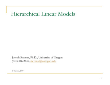
TQMP 2014 vol. 10 no. 1Figure 1 Sample two-level Hierarchical Linear Model.obtains what is called a Level 1 (or within-group)regression equation for each participant, based on thatindividual’s 50 time points (for a total of 100equations); the Level 1 equation may have one or moreLevel 1 independent variables (i.e., independentvariables measured at each time point), or it may haveno independent variables (the same set of independentvariables must be used in all Level 1 equations); thedependent variable must be measured at each timepoint. Like any regression, the Level 1 equation for agiven individual summarizes their data across 50 timepoints into just a few coefficients: an intercept (whichequals the participants’ mean score on the dependentvariable if the researcher uses what is called groupmean centering for each Level 1 independent variable, acommon procedure), and a slope for each of the Level 1independent variables. Each of these coefficients – theintercept and possibly some slopes – then serves as thedependent variable in a Level 2 (or between-group)regression equation; for example, if there are twoindependent variables in the Level 1 equations, therewill be three regression equations at Level 2, onepredicting the Level 1 intercept, one predicting theLevel 1 slope for one Level 1 independent variable, andthe other predicting the slope for the other Level 1independent variable. Each Level 2 equation has anintercept (which equals the mean intercept or slopeacross all participants if the researcher uses what iscalled grand mean centering for each Level 2independent variable, a common procedure), and itmay have one or more Level 2 independent variables(i.e., independent variables measured just once for eachparticipant).For example, suppose again that there are 100participants, with 50 time points each, the dependentvariable is state well-being (s wbeing – HLM truncatesvariable names to eight characters, so you might as wellcreate short names to begin with), the Level 1independent variable is state autonomy (s auton), andthe Level 2 independent variable is trait extraversion(t extrav). Below is what the regression equation lookslike at Level 1. (Note that e is the error term, indicatingthat the observed state well-being score at a given timepoint may differ from the well-being score predicted forthat person based on the regression equation; e isalways present in the Level 1 equation.)The intercept (π0) and the slope (π1) values willdiffer from participant to participant. If state autonomyis group mean centered, the π0 conveniently equals themean well-being score across all time points for a givenparticipant, and thus provides an estimate of theparticipant’s trait level of well-being.Below is what the regression equations look likes atLevel 2. (Note that in HLM, you can choose whether ornot to include the error term r0 and/or r1; if the errorterm r0 is included, this implies that the intercept π0 isassumed to differ from person to person; if the errorterm r1 is included, this implies that the slope π1 isassumed to differ from person to person.)Figure 1 shows a screen shot of how the model wouldappear in HLM.Each equation at Level 2 is a summary across all 100participants, and each of the four coefficients (thoseindicated with the letter β) is tested to determine if itdiffers significantly from zero. If trait extraversion isgrand mean centered, β 00 conveniently equals the meanwell-being score across all time points and across allparticipants, called the grand mean, and thus providesan estimate of the average participant’s trait level ofwell-being. The β 10 value provides the average π1 valueacross all participants (assuming the Level 2independent variable(s) is/are grand mean centered).If β 10 is statistically significant, then on average acrossThe Quantitative Methods for Psychology14
TQMP 2014 vol. 10 no. 1participants, state autonomy significantly relates tostate well-being. The β 01 value gives the relationshipbetween trait extraversion and trait well-being(assuming group mean centering was used). Finally, ifβ11 is significantly different from zero, this indicatesthat trait extraversion moderates the strength of therelationship between state autonomy and state wellbeing (this moderation is also called a cross-levelinteraction, since trait extraversion at Level 2 isinteracting with state autonomy at Level 1; it iscertainly possible to have an interaction betweenindependent variables at the same level, but these areproduct terms that must be created in the data setbefore importation into HLM).When HLM is superior to regular regressionIn the past, before HLM was developed, peoplesimply used a single regular regression for groupeddata – either what is called a Level 1 regression or whatis called a Level 2 regression. Suppose there are 100participants and 50 time points per participant, withthe variables at each level as discussed before. A Level 1regression can be used when the researcher is onlyinterested in relationships at Level 1 (e.g., does stateautonomy relate to state well-being), and it involvessimply running a regression with a sample size of all5000 data points as if they came from 5000independent participants. A Level 2 regression can beused when the researcher is only interested inrelationships at Level 2 (e.g., does trait extraversionrelate to trait well-being), and it involves running aregression on 100 data points, one per participant, aftercomputing the mean well-being score for eachparticipant.The question is: When are these regular regressionsproblematic, making HLM a preferable choice?When HLM is superior to Level 1 regression – theproblem of inflated Type I errorA Level 1 regression treats data from 100 participantsas if it were data from 5000 independent participants.Therein lies the problem. This can lead to a largeinflation of Type I error, since the statistical significanceof a result depends on sample size. HLM deals with thisproblem by basing its sample size for inferentialstatistics on the number of groups (100 in thisexample), not on the total number of observations(5000 in this example).The HLM approach has a drawback of its own, as thereader might guess. HLM tends to be on theconservative side when testing relationships at Level 1,i.e., it has less power than a Level 1 regression would.There usually is some degree of dependence amongthe observations from a given group, however, and it isusually advisable to apply an analysis for grouped data,such as HLM. Only if there is no dependence is itappropriate to conduct a Level 1 regression. It ispossible to determine the degree of within-groupdependence in HLM by testing whether there isvariance in the Level 1 intercept across groups – if itdoes not vary, an analysis for grouped data is notnecessary and one can use a Level 1 regression, thoughone may still want to proceed with an analysis forgrouped data on theoretical grounds or for consistencywith other analyses that are being conducted.Alternatively, an Intraclass Correlation Coefficient (ICC)smaller than 5% suggests that an analysis for groupeddata is unnecessary (Bliese, 2000). The ICC is theproportion of the total variance in the dependentvariable (which is the sum of the between-groupvariance and the within-group variance) that existsbetween groups.When HLM is superior to Level 1 regression – thevalue of differentiating Levels 1 and 2In addition to the reduction of Type I error, there is alsoa conceptual reason to use HLM instead of Level 1regression whenever there is a significant variance incoefficients across groups. HLM allows the researcherto separate within-group effects from between-groupeffects, whereas a Level-1 regression blends themtogether into a single coefficient.For example, in one study, I ran an experiencesampling study with about 100 participants and about50 time points per participant (Huta & Ryan, 2010). AtLevel 1, I measured eudaimonia (the pursuit ofexcellence) and hedonia (the pursuit of pleasure).When I analyzed the data properly, using HLM, Iobtained the following results. At Level 1, so at a givenmoment in time, a person’s degree of state eudaimoniaand state hedonia correlated negatively, around -.3.Thus, if a person is momentarily striving for excellence,they are probably not simultaneously striving forpleasure. However, at Level 2, so at the trait level, aperson’s average degree of eudaimonia over the 50time points and their average degree of hedonia overthe 50 time points actually correlated positively, about.30! Thus, if a person often strives for excellence, theyalso tend to often strive for pleasure. (The latteranalysis was performed by choosing one variable, sayThe Quantitative Methods for Psychology15
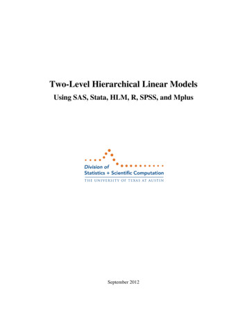
TQMP 2014 vol. 10 no. 1hedoniaCorrect HLMLevel 2 slopei.e., slope betweenpeopleCorrect HLMLevel 1 slopesi.e., slopes within peopleIncorrect Level 1Regression slopemixing between- &within-person slopeseudaimoniaFigure 2 How two variables can have a negative relationship at the within-group level but a positive relationshipat the between-group level in Hierarchical Linear Modeling.hedonia, as the dependent variable for HLM, and then atLevel 2 using each person’s mean eudaimonia score asthe independent variable, with the mean eudaimoniascores being computed for each participant beforerunning the HLM – in other words, HLM can computethe mean score on the dependent variable for eachperson, but the mean score on the independent variablehas to be computed person by person prior to runningHLM). If the data had simply been analyzed using aLevel-1 regression, the correlation between eudaimoniaand hedonia would be -.10, which is part way between .3 and .3 and tells us little about the true correlation atLevel 1 or at Level 2.Figure 2 provides an illustration of how the correctslopes obtained through HLM at Levels 1 and 2 can bein opposite directions from each other, and how theLevel 1 regression slope is a blend of the two slopesobtained through HLM. Each dotted ellipse representsdata across multiple time points for each participants(only three participants are shown). The thin dottedlines running through the dotted ellipses are the linesof best fit for each participant. The thick dotted line isthe mean of all the thin dotted lines across participants,and corresponds to the Level 1 or “within-person”correlation of -.3 I obtained using HLM. The thin solidellipse encompasses all of the data combined acrossparticipants, and the thin solid line is the line of best fitthrough this data and corresponds to the somewhatuninformative correlation of -.1 obtained through aLevel 1 regression. The thick solid line corresponds tothe Level 2 or “between person” correlation of .3obtained using HLM (or using a Level 2 regression), andis the line of best fit through the center points (calledcentroids) of the ellipses for each participant, which areindicated by large dots.When HLM is superior to LevelLevel 2 regressionLet me continue with the example of 100participants and 50 time points per participant, andboth eudaimonia and hedonia being measured at eachtime point. Recall that a Level-2 regression involvestaking the mean dependent variable score and themean independent variable score across the 50 timepoints for each participant, which produces just 100observations in total, and then running a regularregression on those means. The results of a Level 2regression and of HLM will be the same if eachparticipant has the same number of time points and nomissing data (and the same variance in the dependentvariable). But one lovely feature of HLM is that it allowsthe researcher to have different numbers ofobservations per group (i.e., per participant in thisexample) and furthermore gives greater weight to thegroups with more observations (and less variance),which produces slightly more accurate estimates ofpopulation values. The greater the differences insample size (and variance) across groups, the greaterthe advantage of HLM relative to Level-2 regression.This benefit is subtler and less crucial than theadvantage of HLM over Level 1 regression, but it isThe Quantitative Methods for Psychology16
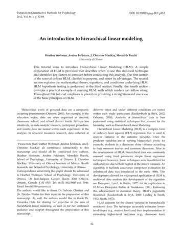
TQMP 2014 vol. 10 no. 1Figure 3 How Functional Data Analysis models the fluctuations a variable undergoes over time.worth being aware of.When it is appropriate to use HLM on data fromdyadsWhen comparing HLM with regular regression, Iwould like to also make a comment about dyads. Dyadsalways have two members per group, e.g., husband andwife, caregiver and patient, coach and athlete. It is acommon assumption that all research on dyads shouldbe analyzed using HLM. This is often true but notalways. HLM only applies when exactly the same set ofvariables – the dependent variable, or the dependentvariable and some Level 1 independent variables – ismeasured in all members of the group, i.e., in bothmembers of the dyad. For example, HLM applies whenthe same marital satisfaction questionnaire is given toboth the husband and the wife. However, if differentvariables have been assessed in the two members of thedyad – for example, if the dependent variable assessedin the caregiver is burnout, but the dependent variableassessed in the patient is depression – then HLM doesnot apply and one would simply run a regularregression (or some other analysis) to predict caregiverburnout, and a separate analysis to predict patientdepression.Different analyses for grouped dataHLM is not the only method available for dealing withgrouped data. The two most common alternatives arestructural equation modeling (SEM) (or its simplerversion, path analysis), and a general linear model(GLM) with a repeated-measures variable, which I willsimply refer to as repeated-measures. Examples of thelatter include: mixed design ANOVA/GLM with arepeated-measures/within-subjects variable that isanalogous to the dependent variable measuredrepeatedly at Level 1 in HLM, and one or morebetween-subjects variables that are analogous to theLevel 2 independent variables in HLM; hin-subjects variable; and a pairedsamples t-test, which has only two repeated measures.A less well-known alternative is functional data analysis(FDA), and there are others still, such as growthmixture modeling (GMM).Let me outline FDA and GMM only briefly, justenough to make the reader aware of these options. Iwill then discuss repeated measures and SEM (and pathanalysis) in more detail, describing how the sameresearch question would be addressed with thesemethods as well as HLM, and listing criteria that canhelp a researcher choose between HLM, repeatedmeasures, and SEM.Functional data analysisDeveloped by Ramsay and Silverman (2002, 2005),FDA is used specifically for longitudinal data. It is moreflexible than other approaches in that it models theprecise pattern of fluctuations that a variableundergoes over time, and every individual/entity canhave a different pattern. This makes FDA more flexiblethan the other approaches I am comparing it with,which assume that a single function (e.g., a straight line,a quadratic curve, a cubic curve, exponential decay) canrepresent the entire span of data points, and that allindividuals can be represented by the same function.For example, Figure 3 shows the pattern of depressionscores over the course of therapy for four individuals. Asmoothing process can then be applied, to a degreegauged by the researcher, in hopes of eliminating minorfluctuations that are likely to represent random noise,and retaining major fluctuations that are likely torepresent a true signal.The Quantitative Methods for Psychology17
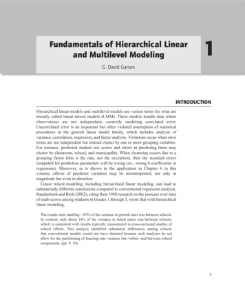
TQMP 2014 vol. 10 no. 1Figure 4 How to set up the Level 1 and Level 2 data sets for Mod
Hierarchical linear modeling (HLM) (also referred to as multilevel modeling, mixed modeling, and random coefficient modeling) is a statistical analysis that many researchers are becoming interested in. Previous publications on HLM have provided d