WIXLIB

Introduction to PredictiveModeling Using GLMsDan Tevet, FCAS, MAAA, Liberty MutualInsurance GroupAnand Khare, FCAS, MAAA, CPCU,Milliman1

Antitrust Notice The Casualty Actuarial Society is committed to adhering strictlyto the letter and spirit of the antitrust laws. Seminarsconducted under the auspices of the CAS are designed solelyto provide a forum for the expression of various points of viewon topics described in the programs or agendas for suchmeetings. Under no circumstances shall CAS seminars be used as ameans for competing companies or firms to reach anyunderstanding – expressed or implied – that restrictscompetition or in any way impairs the ability of members toexercise independent business judgment regarding mattersaffecting competition. It is the responsibility of all seminar participants to be aware ofantitrust regulations, to prevent any written or verbaldiscussions that appear to violate these laws, and toadhere in every respect to the CAS antitrust compliancepolicy.2

A New England vacation The weather The car insurance

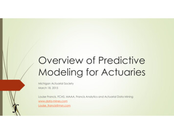
A few words about overfitting The more data we have The more models we have The more sophisticated models become The potential for overfitting data nevergoes away!That’s one big reason to validate models.

In a nutshell0.250.23Prediction error0.21Training data0.190.170.150.130.110.090.070.05Model Complexity Test data

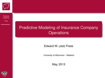
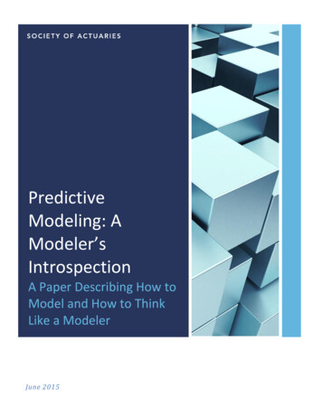
Overfitting U.S. Elections(courtesy of Randall Munroe, writerof “xkcd” and What If)

1876-1944

1948-Present

Outline Overview of predictive modeling Predictive modeling in the actuarial world Simple linear models vs generalized linearmodels (GLMs) Specification of GLMs Interpretation of GLM output Frequency/severity vs pure premium modeling Model validation Modeling process and important considerations The next 100 years9

What is Predictive Modeling Model – an abstraction of reality, generallywith a random or probabilistic component– Simplification of a real world phenomenon Model types include:– Linear models – predict target variable usinglinear combination of predictor variables– Trees – split dataset, one variable at a time, intosubgroups that behave similarly– Neural networks – “self-learning” algorithms thatadapt to best predict a quantity of interest10

How Do Actuaries Use Modeling? Rating plans – model insurance loss data tobuild plans that charge actuarially fair rates Underwriting plans – knowing relative riskinessof policyholder can inform underwriting decisions Enterprise risk management – modelcorrelations between lines of business orprobability of ruin Product analytics – customer retention,conversion, lifetime value11

Simple Linear Model Y β0 β1*X1 β2*X2 ε– Y is the target or response variable – it is what we aretrying to predict (e.g. pure premium)– X1, X2, etc are the explanatory (e.g. age of driver, typeof vehicle) variables – we use them to predict Y– ε is the error or noise term – it is the portion of Y thatis unexplained by X μ E(Y) β0 β1*X1 β2*X2 βn*Xn In general, we are modeling the mean of Y12

Simple Linear Model Assumptions Assumptions of simple linear models– Target variable Y does not depend on the value of Y forany other record, only the predictors– Y is normally distributed– Mean of Y depends on the predictors, but all records havesame variance– Y is related to predictors through simple linear function Unfortunately, these assumptions are oftenunrealistic– Target variables of interest, such as pure premium,frequency, and severity, are not normally distributed andhave non-constant variance13

Generalized Linear Models Generalized linear model: g( ) β0 β1*X1 β2*X2 βn*Xn Assumptions of generalized linear models– Target variable Y does not depend on the value of Y forany other record, only the predictors– Distribution of Y is a member of the exponential family ofdistributions– Variance of Y is a function of the mean of Y– g( ) is linearly related to the predictors. The function g iscalled the link function The exponential family of distributions include thefollowing: Normal, Poisson, Gamma, Binomial,Negative Binomial, Inverse Gaussian, Tweedie14

GLM Variance Function Var(Y) φ*V(μ)/w φ is the dispersion coefficient, which isestimated by the GLM w is the weight assigned to each record– GLMs calculate the coefficients that maximizelikelihood, and w is the weight that each record getsin that calculation V(μ) is the GLM Variance Function, and isdetermined by the distribution– Normal: V(μ) 1– Poisson: V(μ) μ– Gamma: V(μ) μ215

GLM Link Function g(μ) β0 β1*X1 β2*X2 Common choices for link function– Identity: g(μ) μ– Log: g(μ) ln(μ)– Logit: g(μ) ln(μ/(1- μ)) Log link commonly used to model rating plansbecause it produces multiplicative relativities– ln(μ) β0 β1*X1 β2*X2 μ exp(β0 β1*X1 β2*X2) μ exp(β0)*exp(β1*X1) *exp(β2*X2) Logit link used to model probability of anevent occurring16

Offsets An effect in a model that is fixed by the modeler Variable offsets – fix the effect of variables that arenot being modeled– Example: Constructing a rating plan and not modeling baseterritory rates– Solution: Offset for current territory rates Volume offsets – reflect fact that different recordshave different volumes of data and thus havedifferent expected values– Example: Modeling claim counts. Some records have a singleexposure, other have many exposures– Solution: Offset for exposure volume of each observation17

Interpreting GLM Coefficients w/ Log Link Discrete variables: exponentiate GLM coefficient– Example: coefficient for youth drivers is 0.52 Rating factor exp(0.52) 1.68 Youth drivers have 68% surcharge relative to base level of adultdrivers (who, by definition, have rating factor of 1.00) Continuous variables with no transformation– Example: modeling pure premium, and annual miles driven is acontinuous variable– As miles driven increases by 1 unit, expected pure premium is scaled bya factor of exp(β), regardless of whether mileage goes from 1,000 to2,000 or 20,000 to 21,000 Continuous variables with log transformation– Pure premium (annual mileage) β– If β 1, then as mileage increases, pure premium increases atdecreasing rate18

Uncertainty in Parameter Estimates GLMs allow us to quantify uncertainty in parameterestimates Wald 95% confidence interval for mean ofparameter estimate Mean /- 1.96*(StandardError) Test for the significance of an individual parameter– Wald Chi Square (Parameter Estimate/Standard Error) 2Approximately follows a Chi Squared distribution with 1 degreeof freedom– P-value is probability of obtaining a Chi Square statistic of givenmagnitude by pure chanceLower p-value more significant19

Two Modeling Approaches Pure Premium Approach: Build a single model forpure premium– Generally straightforward to implement Frequency-Severity Approach: Build one model forclaim frequency and another for claims severity– Additional work for additional insight20

Pure Premium Approach Advantages:– Only a single model needs to be built– No need to split variable offsets– Results often very similar to frequency-severity approach Disadvantages:– Yields less insight than frequency-severity– Tweedie distribution is only good choice Relatively new and mathematically complex Includes implicit assumptions that may not hold21

Frequency-Severity Approach Advantages:– May yield meaningful insights about data– Can choose from several well-known and wellunderstood distributions Disadvantages:– Two models to build, run, and validate– Requires splitting variable offsets– Often produces limited additional benefit22

Tweedie Distribution Mixed Poisson-Gamma process – number ofclaims follow a Poisson distribution, and the sizeof each claim follows a Gamma distribution The Tweedie is a 3-parameter distribution:– Mean (μ), equal to the product of the means of theunderlying Poisson and Gamma distributions– Power (p), which depends on the coefficient ofvariation of the underlying Gamma distribution– Dispersion (φ), a measure of variance23

Frequency Distribution Options Poisson– The Coca Cola of claim count distributions Overdispersed frequency distributions– Overdispersed Poisson– Zero-Inflated Poisson– Negative Binomial– Zero-Inflated Negative Binomial24

Severity Distribution Options Several reasonable distributions Criteria– Member of exponential family– p 2, where V(µ) µp In order of increasing variance:––––Gamma (p 2)Tweedie (2 p 3)Inverse Gaussian (p 3)Tweedie (p 3)25

Three Pillars of Model Validation Tests of Fit Tests of Lift Tests of Stability26

Fit Statistics Traditional: Absolute/Squared Error Alternatives: Likelihood, Deviance, Pearson’sChi-Squared Penalized: AIC, BIC Per Observation: Residuals, Leverage27

Absolute/Squared Error Only appropriate if data is normally distributed Inappropriate to use on disaggregate claimfrequency, severity, or pure premium data Useful to assess model fit within buckets– Bucket data into percentiles, or similar quantiles, andcalculate squared difference between actual andpredicted for each bucket28

Better Alternatives to Squared Error Likelihood: chance of observation, given model– Always increases as parameters are added to model Deviance: twice the difference in loglikelihoodsbetween the saturated and fitted models– GLMs are fit so as to minimize deviance– Accounts for the shape of the distribution Pearson’s chi-squared: squared error divided bythe variance function of the distribution– Accounts for the skew of the distribution29

Penalized Measures Akaike Information Criterion (AIC): Penalizesloglikelihood for additional model parameters Bayesian Information Criterion (BIC): Penalizesloglikelihood for additional model parameters, andthis penalty increases as the number of records inthe dataset increases– Can be too restrictive Used primarily for variable selection30

Per Observation Traditional residual: actual minus predicted Deviance residual: square root of weighteddeviance times sign of actual minus predicted– Reflects the shape of the distribution– Plotting deviance residual against weight or anypredictor should yield an uninformative cloud– Should be approximately normally distributed Leverage: used to identify extreme outliers– Does not necessarily measure impact31

Model Lift Lift is meant to approximate economic value– Fit has no relationship with economic value Economic value is produced by comparativeadvantage in avoidance of adverse selection– Lift is a comparative measure, i.e. the lift of one modelover another, or the lift of a model over status quo Lift should always be measured on holdout data32

Lift Measures Simple Quantile PlotDouble Lift ChartLoss Ratio ChartGini Index33

Model Lift – Simple Quantile Plots34

Double Lift Chart35

Loss Ratio Chart36

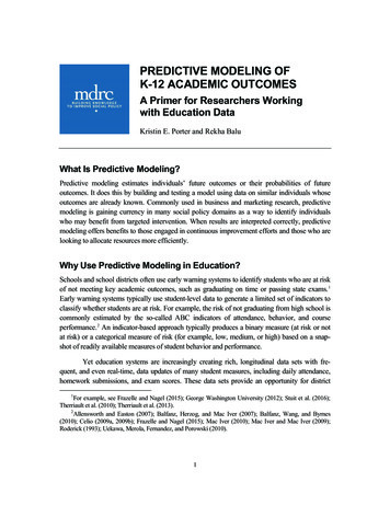
Economic Gini Index37

Gini Index of Rating Plan Model should differentiate lowest and highest losscost policyholders Creation of Gini index:– Order policyholders by model prediction, from best toworst– X-axis is cumulative percent of exposures– Y-axis is cumulative percent of losses Had model produced Gini index in prior slide, wouldhave identified 60% of exposures that contributeonly 20% of losses38

Methods for Testing Model Stability Cross-validation– Split data into subsets (e.g. by time period)– Refit model on each subset– Compare model parameter estimates Bootstrapping– Refit model on many bootstrapped samples– Calculate variability of parameter estimates Deletion of influential records39

Measures of Influence Cook’s Distance: Statistical measure of theimpact each record has on the overall model– Excellent tool for identifying errors or anomalies– Deletion of records with high Cook’s Distancemay significantly change model results, and sothis procedure can be used to test stability DFBETA: Influence on a certain parameter Influence is not to be confused with leverage40