Transcription
PredictiveModeling: AModeler’sIntrospectionA Paper Describing How toModel and How to ThinkLike a ModelerJune 2015
Predictive Modeling: A Modeler’sIntrospectionA Paper Describing How to Model and How to Think Like a ModelerSPONSORSCommittee on Finance ResearchAUTHORSMichael Ewald, FSA, CFA, CERAQiao WangCAVEAT AND DISCLAIMERThe opinions expressed and conclusions reached by the authors are their own and do not represent any official position oropinion of the Society of Actuaries or its members. The Society of Actuaries makes not representation or warranty to theaccuracy of the information.Copyright 2015 All rights reserved by the Society of Actuaries
AcknowledgementsThe authors would like to express their gratitude to the SOA Project Oversight Group. The quality of thispaper has been enhanced through their valuable input. The group includes the following individuals:William Cember, Andy Ferris, Jean-Marc Fix (chair), John Hegstrom, Christine Hofbeck, Steve Marco,Dennis Radliff, Barbara Scott (SOA), and Steven Siegel (SOA).Additionally, we would like to thank our colleagues and friends: Andrew Dalton, Katherine Ewald, JimKing, Alex Marek, and Tom Tipton. We could not have produced this paper without their help andfeedback. Additionally, they have helped make us better modelers, actuaries, and people. Society of Actuaries, All Rights ReservedMichael EwaldPage 1
Table of ContentsIntroduction – Historical Actuarial Approach . 4GLM Overview. 5The Math . 6Applications. 7Good Models. 9Data Overview. 10Modeling Process . 11Project Scope . 11Data Collection . 12Data Scope . 12Data Structure . 13Data Scrubbing . 13Data Preparation . 14Variable Transformations. 14Variable Grouping . 15Separating Datasets . 15Building a Model . 17Defining the Distribution . 17Fitting Main Effects . 18Grouping Main Effects . 23Significance of Levels . 23Counterintuitive Signals . 25Parameter Confidence Intervals . 26Variates . 28Mid-Model Grouping . 31Control Variables. 31Interactions . 32Model Validation. 34Parameterize Model on the Test Dataset . 34Compare Train and Test Factors . 35 Society of Actuaries, All Rights ReservedMichael EwaldPage 2
Offset Train Model and Score on the Test Dataset. 37Backwards Regression. 37Model Evaluation . 38Gini . 38Out-of-Time. 38Decile Charts . 39Combining Models . 40Selection and Dislocation . 41Selection. 41Dislocation . 42Implementation . 43Documentation . 43Monitoring/Reporting . 43Conclusion . 44 Society of Actuaries, All Rights ReservedMichael EwaldPage 3
Introduction – Historical Actuarial ApproachInsurance practitioners have been analyzing risk for thousands of years. From the Code ofHammurabi, which waived loans on a ship if it was lost in voyage, to the initial mortality tablesdeveloped by John Graunt in the mid-18th century1, the goal of the actuary has remainedconstant: analyze “the financial consequences of risk.”2 As society has progressed andtechnology has developed, both the design of insurance products and the means of analyzing therisk have increased in complexity. The introduction of computers has, in a very short period oftime, changed the way actuaries approach their day-to-day jobs. The need for both technical andproduct expertise has never been greater. The goal of this paper is to help you understand onetool that has gained an enormous amount of traction over the past two decades: predictivemodeling. Predictive modeling is the practice of leveraging statistics to predict outcomes. Thetopic covers everything from simple linear regression to machine learning. The focus of thispaper is a branch of predictive modeling that has proven extremely practical in the context ofinsurance: Generalized Linear Models (GLMs).Before moving to GLMs, it is important to understand actuarial techniques that have been usedin the past. In particular, we will discuss one and two-way analysis. Although the terminologymay be foreign, anyone with a basic analytical background has used these techniques. One-wayanalysis refers to the review of a response by a single variable (e.g. observed mortality by age).Two-way analysis looks at the response by two variables (e.g. observed mortality by age andgender). Relativities between variable groupings are then used to ascertain the risk between thetwo groups (i.e. mortality of a 46 year old male versus that of a 45 year old male). Thistechnique is then applied to other variables to help segment the risk in question. Although thistechnique is extremely intuitive, it has a number of well-known drawbacks:---12Ignores correlations - If Detroit experience is 20% worse than average and if automanufacturing segment experience is 20% worse than average, should we expect automanufacturers in Detroit to have experience that is 40% worse than average?Suffers from sequencing bias - The first variable analyzed may account for the signal ofvariables that will be analyzed later. This could reduce or eliminate the importance ofthose variables.Cannot systematically identify noise – One large claim or a large unique policy can havea very large impact on one-way analyses. It is difficult to identify the signal (true impactof a variable) vs. noise (volatility) in one-way analyses.Klugman, Stuart A., “Understanding Actuarial Practice,” Society of Actuaries, 2012, Page 7.Society of Actuaries. 2010. “What is an Actuary?” .aspx. Society of Actuaries, All Rights ReservedMichael EwaldPage 4
Although actuaries have developed techniques to account for these pitfalls, they are timeconsuming and require substantial judgment. GLMs provide a systematic approach thataddresses the above concerns by allowing all variables to be analyzed in concert.GLM OverviewLet us begin with normal linear regression. Most readers will be familiar with this form of GLM.It is well known that linear models, along with all GLMs, require independence of observations.There are three assumptions unique to linear regression that we address below3:1. Error terms follow normal distribution2. Variance is constant3. The covariates effect on the response are additiveThese assumptions are relaxed when reviewing GLMs. The new assumptions are as follows4:1. Error term can follow a number of different distributions from the exponential family2. Variance does not need to be constant3. The covariates can be transformed so that their effect is not required to be additive.Relaxing the first assumption allows us to utilize exponential distributions that apply directly tothe insurance industry. For distributions that are strictly non-negative, such as claims, a normaldistribution that exists across all real numbers is not ideal. The Poisson distribution and Gammadistribution apply to only positive numbers and are more appropriate for claim counts and claimamounts, respectively. The Binomial distribution applies to all binary datasets, and may beappropriate for modeling policyholder behavior or mortality.GLMs allow variance to adjust with the mean. As you can see in the exhibit below, the varianceof the Poisson and Gamma distributions increase as their means (1-p)Normalµσ2Poisson2There are many instances where this makes intuitive sense. When modeling claim amounts, weexpect absolute variability to increase as the dollars increase. Additionally, when reviewing thebinomial variance formula, variance approaches zero as the mean tends toward zero or one.53McCullagh, P. and J. A. Nelder, “Generalized Linear Models”, 2nd Edition, Chapman & Hall, CRC, 1989. Pages 23.McCullagh, P. and J. A. Nelder, “Generalized Linear Models”, 2nd Edition, Chapman & Hall, CRC, 1989. Pages 31.5McCullagh, P. and J. A. Nelder, “Generalized Linear Models”, 2nd Edition, Chapman & Hall, CRC, 1989. Pages 12.4 Society of Actuaries, All Rights ReservedMichael EwaldPage 5
Finally, the assumption of additive covariates is neither intuitive, nor can it be easily applied toactuarial analyses. Predictive modeling allows this assumption to be relaxed. For example, riskfactors can be multiplicative. This is extremely useful when developing a pricing algorithm thatfollows a manual rate structure.The MathBefore addressing the calculations to develop a model, it is important to understand the structureof the final equation. There are three main components of both normal linear regression andGLMs:1. Random Component – distribution of the error term.2. Systematic Component – summation of all covariates (i.e. predictors) that develop thepredicted value.3. Link Function – relates the linear predictor to the expected value of the dataset. In otherwords, it is a mathematical transformation of the linear predictor that allows the expectedmean to be calculated.The linear regression model is as follows:𝐸 [𝑌𝑖 ] 𝛽0 𝛽1 𝑥𝑖,1 𝛽2 𝑥𝑖,2 𝛽𝑛 𝑥𝑖,𝑛 𝜀𝑖SystematicComponentRandomComponentThe formula above shows the expected value of each observation i. This is calculated bymultiplying a vector of rating variables B and a vector of observed values X. The notation willmake more sense in later sections when these formulas are applied to real life scenarios. Inlinear regression, the expected value is equal to the systematic component because the identitylink (described below) does not transform the systematic component.When moving to a GLM, the random component can take on a member of the exponential familyand the systematic component is transformed via a link function:𝐸 [𝑌𝑖 ] 𝑔 1 (𝛽0 𝛽1 𝑥𝑖,1 𝛽2 𝑥𝑖,2 𝛽𝑛 𝑥𝑖,𝑛 ) 𝜀𝑖Link Function Society of Actuaries, All Rights ReservedSystematicComponentRandomComponentMichael EwaldPage 6
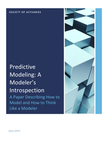
The link function is simply an algebraic transformation of the systematic component. Please seethe applications section below for examples of the link function.Now that we have seen what we are working towards, let us discuss how we develop the finalformula. GLMs develop parameters in such a way that minimizes the difference between actualand predicted values. In linear regression, parameters are developed by minimizing the sum ofsquared errors. The same result can be achieved through maximum likelihood estimation(MLE). MLEs are used to parameterize GLMs.For any member of the exponential family there exists a density function: 𝑓(𝑦; 𝜃). Taking thelog of each density function for each observation and adding them together gives the loglikelihood function.6𝑙(𝜇; 𝑦) log 𝑓𝑖 (𝑦𝑖 ; 𝜃𝑖 )𝑖To calculate the parameters, take the derivative of the likelihood function with respect to therating variables and set them to zero: 𝑙 0 𝛽1 𝑙 0 𝛽2. 𝑙 0 𝛽𝑛Using these equations, you then solve for the parameters in question.ApplicationsDistributionsThe type of GLM chosen for a project hinges on the distribution of the data. The table belowdetails the major distributions.7The table below details the canonical link for some common distributions. The canonical link isthe link that can be used to calculate the parameters in closed form. Given the size of modeling67McCullagh, P. and J. A. Nelder, “Generalized Linear Models”, 2nd Edition, Chapman & Hall, CRC, 1989. Page 24.McCullagh, P. and J. A. Nelder, “Generalized Linear Models”, 2nd Edition, Chapman & Hall, CRC, 1989. Page 30. Society of Actuaries, All Rights ReservedMichael EwaldPage 7
datasets, parameters are never calculated in this manner. They are calculated using numericalmethods (i.e. an iterative process). Since the canonical link is not a requirement to parameterizethe model, other link functions may be chosen if they are more practical.Range of y Canonical Linkidentityθ1Poisson 0, 1, logexp(θ)µBinomial0, 1logiteθ/(1 eθ)µ(1 - µ)Gamma(0, )reciprocal*1/θµ2Normal(- , )E(Y;θ) Var Function* Gamma distribution often uses log link function for easierimplementation. This is explained in more detail insubsequent sections.The name of the link functions and their transformations are described in the “Canonical Link”and “E(Y;θ)” columns. For example, the binomial distribution uses the logit link. Thetransformation is as follows:𝑒 𝑆𝑦𝑠𝑡𝑒𝑚𝑎𝑡𝑖𝑐 𝐶𝑜𝑚𝑝𝑜𝑛𝑒𝑛𝑡1 𝑒 𝑆𝑦𝑠𝑡𝑒𝑚𝑎𝑡𝑖𝑐 𝐶𝑜𝑚𝑝𝑜𝑛𝑒𝑛𝑡Normal: The normal distribution is useful for modeling any response that exists betweennegative and positive infinity. It can be used in an analysis focused on changes in a variable.For example, one might want to look at the drivers of changes in premium. This practice is alsoknown as premium dislocation.Poisson: The Poisson distribution is primarily used to model claim counts when multiple claimscan occur in a given exposure period. For example, a policyholder with health care coverage canhave multiple physician claims in a given month. The Poisson distribution is also useful whenmodeling claims in group insurance, because claim counts may be reviewed at the group levelrather than the individual level.Binomial: The binomial distribution can be used to model binary responses. Examples in aninsurance context are as follows:-Mortality – the probability of dying.Lapse/persistency – probability of a policyholder/client retaining or cancelling theircoverage.Close ratio/issue rate – probability of selling a policy.Annuitization – probability of a policyholder annuitizing a contract. Society of Actuaries, All Rights ReservedMichael EwaldPage 8
-Termination/recovery – probability a claimant currently on disability will recover and theclaim will terminate. This can be used to develop reserve assumptions.The binomial distribution is by no means limited to the examples above. The distribution can beused for any other situation characterized by a binary response. Moreover, non-binary data canbe transformed into a binary distribution to develop meaningful analytics. For example, whenreviewing large claim amounts, you can create a binary distribution that looks at claims greaterthan a certain threshold to determine the characteristics of those claims.Gamma: The gamma distribution is most often used for claim severity (i.e. claim amount givena claim has occurred). The gamma distribution is appropriate to handle the long tailed nature ofclaim amounts. Additionally, it can be used to model pure premium (loss costs excludingoverhead and profit loading).Tweedie: Although not shown in the table above, the Tweedie distribution is very useful in bothP&C and Group insurance. The Tweedie distribution is a hybrid between the Poisson andGamma distributions. Therefore, it is applicable to pure premium and loss ratio modeling. Lossratio modeling determines what variables cause deviation from the average loss ratio. For caseswith minimal exposures, there is high probability of zero claims and a loss ratio of zero. TheTweedie distribution, with a point-mass at zero and a long tail, is perfect for this type of analysis.We detail the common distributions and their potential uses below:Potential ModelsLink FunctionNormal Dislocation (i.e. Change in Premium)identityPoisson Claim Frequency (incidence)logMortality RatesLapse/Persistency RatesBinomial Close Ratio/Issue RateslogitAnnuitization RatesTermination/Recovery RatesClaim SeverityGammalog*Pure PremiumPure PremiumTweedielogLoss Ratio Modeling* Gamma distribution often uses log link function rather than the reciprocal link.This is explained in more detail in subsequent sections.Good ModelsChoosing the appropriate distribution is paramount when embarking on a modeling project.However, choosing an appropriate distribution does not necessarily lead to a good model. Themodeler will utilize historical information to inform decisions regarding future events. A good Society of Actuaries, All Rights ReservedMichael EwaldPage 9
model will reflect historical information expected to persist in the future and control forhistorical anomalies. This involves avoiding two opposing modeling risks: overfitting andunderfitting.Overfitting occurs when a model does a good job of predicting the past, but a poor job ofpredicting the future. An extreme example of overfitting is creating a model with as manyparameters as observations. The model would predict the past perfectly, but it would not providemuch insight to future.8Underfitting does a good job of predicting the future on average, but does not do a good job ofsegmenting risk factors. An extreme example is a model with one parameter: the average of thepast.The modeling process discussed in subsequent sections will help the reader avoid bothoverfitting and underfitting. Other principles mentioned in the Generalized Linear Modeltextbook by P. McCullagh and J. A. Nelder are as follows9:1. “ all models are wrong; some, though, are more useful than others and we should seekthose.”2. Do not “ fall in love with one model to the exclusion of alternatives.”3. The modeler should perform “ thorough checks on the fit of a model.”The first principle lays the groundwork for a skepticism that all modelers should possess. Thepopularity of modeling, driven by the results it has produced over the past decade, leads mostindividuals to give significant (and possibly too much) credence to the practice. Although it is avery powerful tool, modeling is only as good as the modeler’s ability to take past data and informmeaningful future results.The second point explains that modeling may not always be the best solution. Time constraints,lack of data, lack of resources, etc. are all impediments to developing a good model. Do notblindly choose a predictive model without understanding the costs and benefits.The final point will be discussed further in the “Model Validation” section.Data OverviewThe first, and arguably the most important aspect of predictive modeling is data preparation. Weoften call this “the 80%” because 80% of the time will be spent preparing the data and 20% willbe spent building and checking the model. This is not a strict rule. Given that the majority of theauthors’ work has been the first of its kind, data preparation is very time consuming. Ascompanies focus more and more on “model ready data,” the goal is that data preparation will89McCullagh, P. and J. A. Nelder. “Generalized Linear Models.” 2nd Edition. Chapman & Hall, CRC. 1989. Page 7.McCullagh, P. and J. A. Nelder, “Generalized Linear Models”, 2nd Edition, Chapman & Hall, CRC, 1989. Page 8. Society of Actuaries, All Rights ReservedMichael EwaldPage 10
take 20% of the time and modeling will take 80%, with the absolute amount of time per projectdecreasing substantially.The modeling dataset consists of rows, which are observations. Each observation will have acorresponding exposure or exposure unit (i.e. weight). Depending on the dataset, observationsmay equal exposures. For example, an individual life mortality study may have a row for eachlife month. In this case, the number of observations equals the number of exposures. In otherinstances, exposures will differ from observations. In a loss ratio model, which compares claimamounts to premium for clients over a period of time, the exposure would be the premium paidin the period that corresponds to the claim amounts.The dataset columns consist of three sections: response, weight, and variables. The responsefield is also referred to as the dependent variable. The dependent variable is what you are tryingto model, and the independent variables are what you are using to predict the dependent variable.The weight defines the exposure (i.e. credibility) of each observation. The more weight of anobservation means it will have a larger impact on the final parameters than an observation withless weight. The independent variables (variables 1, 2, 3, etc.) in the exhibit below are what willbe tested for their predictive power; they are often referred to as covariates.Response WeightVariable 1 Variable 2 Variable 3 Variable nObservation 1Observation 2Observation3.Observation nModeling ProcessProject ScopeLaying out the initial project scope is imperative for any modeling project. This is mostimportant when embarking on a predictive model for the first time. Interested in your new work,your business partners will probably ask for additional analysis. Sticking to a pre-defined scopewill limit project creep and allow you to meet your deliverables in a timely manner.Modeling Participants:Modeling Team - Modeling experts- Need strong data and business knowledge- Have business knowledge (product, claims,Businessunderwriting, sales, etc.) of data and businessPartnersprocess- Owners of the final model Society of Actuaries, All Rights ReservedMichael EwaldPage 11
ITProjectManager- Their involvement in the process helps thembetter understand and support the final model- Advocate your model across organization- Produce initial dataset- Implement final model- Provide management expertise, allowingother participants to spend time moreefficientlyWhile setting scope, it is important to define the relationships with project participants,especially IT. When dealing with large amounts of unstructured data, IT will be an importantresource for both acquiring and understanding the data. All too often, data is assumed to beclean. However, the modeler should understand that data is often entered by individuals whosegoals are not necessarily aligned with the most accurate model data. Underwriters, salesrepresentatives, and clients are often the major suppliers of data.Given outdated IT systems, constraints, and other impediments, these business partners mayenter information that results in the correct answer in their context, but that does not lead toaccurate data. Group life insurance provides a good example. Benefit amounts can be defined aseither flat or a multiple of salary. If a policyholder chooses a flat benefit and salary is not ratebearing, the underwriter may enter the flat benefit amount as the salary. Although this has noprice implications, it would make it difficult for the modeler to understand the true impact ofsalary on mortality. In group insurance, we check the percent of people with the same “salary.”If this number is large, the underwriter most likely entered a flat benefit amount for eachindividual. This data should be segregated from the true salary data. It may be useful to includesales and underwriting in portions of this process to better understand the data.Along with the benefit of understanding data, including representatives from sales, underwriting,and other users of your model may have other benefits. If sales will be impacted, it is importantto include them in the process so that they are aware of what is changing and why. If they feelincluded, they will be advocates for you and will help socialize the changes with the field. Thismust be delicately balanced with the risk of having too many people involved. The modelingteam and business partners must decide the best means of balancing the pros and cons ofincluding groups affected by the project. Depending on the scope of the project, other businesspartners may include, but are not limited to, claims, ERM, marketing, and underwriting staff.Data CollectionData ScopeThe first step when compiling a dataset is to determine the scope of variables that will be testedin the model. Naturally, you will want to test internal data sources. Additionally, you may wantto leverage external data to supplement the internal data. Common sources include government Society of Actuaries, All Rights ReservedMichael EwaldPage 12
data, credit data, social networking websites, Google, etc. This data is commonly acquiredthrough third party data aggregators, including Experian, Axiom, D&B, and others. Externaldata can also be used to inform data groupings or as a proxy for other variables, such as ageographic proxy. Additionally, external data can be combined with internal data to createinteresting variables. For example, you could combine salary and median income in a region tocontrol for cost of living across regions. A 100,000 salary in New York City leads to a verydifferent lifestyle than 100,000 in North Dakota.It is important to avoid preconceived notions when constructing the dataset. Including as muchinformation (where practical) in the beginning will allow for the most meaningful analysis. Morevariables generally lead to more “a-ha” moments. Additionally, there is very little harmincluding additional data fields, because the modeli
modeling. Predictive modeling is the practice of leveraging statistics to predict outcomes. The topic covers everything from simple linear regression to machine learning. The focus of this paper is a branch of predictive modeling that has proven extremely practical in the context of insurance: Generalized Linear Models (GLMs).File Size: 1MBPage Count: 46