Transcription
INTRODUCTION TO BAYESIAN ANALYSISArto LuomaUniversity of Tampere, FinlandAutumn 2014Introduction to Bayesian analysis, autumn 2013University of Tampere – 1 / 130
Who was Thomas Bayes?Basic plemultiparametermodelsMarkov chainsMCMC methodsModel checkingand comparisonHierarchical andregressionmodelsCategorical dataThomas Bayes (1701-1761) was an English philosopher andPresbyterian minister. In his later years he took a deep interest inprobability. He suggested a solution to a problem of inverseprobability. What do we know about the probability of success if thenumber of successes is recorded in a binomial experiment? RichardPrice discovered Bayes’ essay and published it posthumously. Hebelieved that Bayes’ Theorem helped prove the existence of God.Introduction to Bayesian analysis, autumn 2013University of Tampere – 2 / 130
Bayesian paradigmBasic esian paradigm:posterior information prior information data informationSimplemultiparametermodelsMarkov chainsMCMC methodsModel checkingand comparisonHierarchical andregressionmodelsCategorical dataIntroduction to Bayesian analysis, autumn 2013University of Tampere – 3 / 130
Bayesian paradigmBasic plemultiparametermodelsMarkov chainsMCMC methodsModel checkingand comparisonHierarchical andregressionmodelsBayesian paradigm:posterior information prior information data informationMore formally:p(θ y) p(θ)p(y θ),where is a symbol for proportionality, θ is an unknownparameter, y is data, and p(θ), p(θ y) and p(y θ) are the densityfunctions of the prior, posterior and sampling distributions,respectively.Categorical dataIntroduction to Bayesian analysis, autumn 2013University of Tampere – 3 / 130
Bayesian paradigmBasic plemultiparametermodelsMarkov chainsMCMC methodsModel checkingand comparisonHierarchical andregressionmodelsCategorical dataBayesian paradigm:posterior information prior information data informationMore formally:p(θ y) p(θ)p(y θ),where is a symbol for proportionality, θ is an unknownparameter, y is data, and p(θ), p(θ y) and p(y θ) are the densityfunctions of the prior, posterior and sampling distributions,respectively.In Bayesian inference, the unknown parameter θ is consideredstochastic, unlike in classical inference. The distributions p(θ)and p(θ y) express uncertainty about the exact value of θ. Thedensity of data, p(y θ), provides information from the data. Itis called a likelihood function when considered a function of θ.Introduction to Bayesian analysis, autumn 2013University of Tampere – 3 / 130
Software for Bayesian StatisticsBasic plemultiparametermodelsMarkov chainsMCMC methodsIn this course we use the R and BUGS programming languages.BUGS stands for Bayesian inference Using Gibbs Sampling.Gibbs sampling was the computational technique first adoptedfor Bayesian analysis. The goal of the BUGS project is toseparate the ”knowledge base” from the ”inference machine”used to draw conclusions. BUGS language is able to describecomplex models using very limited syntax.Model checkingand comparisonHierarchical andregressionmodelsCategorical dataIntroduction to Bayesian analysis, autumn 2013University of Tampere – 4 / 130
Software for Bayesian StatisticsBasic plemultiparametermodelsMarkov chainsMCMC methodsModel checkingand comparisonHierarchical andregressionmodelsCategorical dataIn this course we use the R and BUGS programming languages.BUGS stands for Bayesian inference Using Gibbs Sampling.Gibbs sampling was the computational technique first adoptedfor Bayesian analysis. The goal of the BUGS project is toseparate the ”knowledge base” from the ”inference machine”used to draw conclusions. BUGS language is able to describecomplex models using very limited syntax.There are three widely used BUGS implementations:WinBUGS, OpenBUGS and JAGS. Both WinBUGS andOpenBUGS have a Windows GUI. Further, each engine can becontrolled from R. In this course we introduce rjags, the Rinterface to JAGS.Introduction to Bayesian analysis, autumn 2013University of Tampere – 4 / 130
Contents of the courseBasic plemultiparametermodelsMarkov chainsBasic conceptsSingle-parameter modelsHypothesis testingSimple multiparameter modelsMarkov chainsMCMC methodsModel checkingand comparisonMCMC methodsHierarchical andregressionmodelsModel checking and comparisonHierarchical and regression modelsCategorical dataCategorical dataIntroduction to Bayesian analysis, autumn 2013University of Tampere – 5 / 130
Basic conceptsBayes’ theoremExamplePrior andposteriordistributionsExample 1Example 2Decision theoryBayes estimatorsExample 1Example 2Conjugate priorsNoninformativepriorsIntervalsPredictionBasic plemultiparametermodelsMarkov chainsMCMC methodsModel checkingand comparisonIntroduction to Bayesian analysis, autumn 2013University of Tampere – 6 / 130
Bayes’ theoremBasic conceptsBayes’ theoremExamplePrior andposteriordistributionsExample 1Example 2Decision theoryBayes estimatorsExample 1Example 2Conjugate priorsNoninformativepriorsIntervalsPredictionLet A1 , A2 , ., Ak be events that partition the sample space Ω,(i.e. Ω A1 A2 . Ak and Ai Aj when i 6 j) and letB an event on that space for which Pr(B) 0. Then Bayes’theorem isPr(Aj ) Pr(B Aj )Pr(Aj B) Pkj 1 Pr(Aj ) Pr(B Aj tiparametermodelsMarkov chainsMCMC methodsModel checkingand comparisonIntroduction to Bayesian analysis, autumn 2013University of Tampere – 7 / 130
Bayes’ theoremBasic conceptsBayes’ theoremExamplePrior andposteriordistributionsExample 1Example 2Decision theoryBayes estimatorsExample 1Example 2Conjugate e-parametermodelsHypothesistestingLet A1 , A2 , ., Ak be events that partition the sample space Ω,(i.e. Ω A1 A2 . Ak and Ai Aj when i 6 j) and letB an event on that space for which Pr(B) 0. Then Bayes’theorem isPr(Aj ) Pr(B Aj )Pr(Aj B) Pkj 1 Pr(Aj ) Pr(B Aj ).This formula can be used to reverse conditional probabilities. Ifone knows the probabilities of the events Aj and theconditional probabilities Pr(B Aj ), j 1, ., k, the formula canbe used to compute the conditinal probabilites Pr(Aj B).SimplemultiparametermodelsMarkov chainsMCMC methodsModel checkingand comparisonIntroduction to Bayesian analysis, autumn 2013University of Tampere – 7 / 130
Example (Diagnostic tests)Basic conceptsBayes’ theoremExamplePrior andposteriordistributionsExample 1Example 2Decision theoryBayes estimatorsExample 1Example 2Conjugate priorsNoninformativepriorsIntervalsPredictionA disease occurs with prevalence γ in population, and θindicates that an individual has the disease. HencePr(θ 1) γ, Pr(θ 0) 1 γ. A diagnostic test gives aresult Y , whose distribution function is F1 (y) for a diseasedindividual and F0 (y) otherwise. The most common type of testdeclares that a person is diseased if Y y0 , where y0 is fixed onthe basis of past multiparametermodelsMarkov chainsMCMC methodsModel checkingand comparisonIntroduction to Bayesian analysis, autumn 2013University of Tampere – 8 / 130
Example (Diagnostic tests)Basic conceptsBayes’ theoremExamplePrior andposteriordistributionsExample 1Example 2Decision theoryBayes estimatorsExample 1Example 2Conjugate e-parametermodelsHypothesistestingA disease occurs with prevalence γ in population, and θindicates that an individual has the disease. HencePr(θ 1) γ, Pr(θ 0) 1 γ. A diagnostic test gives aresult Y , whose distribution function is F1 (y) for a diseasedindividual and F0 (y) otherwise. The most common type of testdeclares that a person is diseased if Y y0 , where y0 is fixed onthe basis of past data. The probability that a person isdiseased, given a positive test result, isPr(θ 1 Y y0 )γ[1 F1 (y0 )]. γ[1 F1 (y0 )] (1 γ)[1 F0 (y0 )]SimplemultiparametermodelsMarkov chainsMCMC methodsModel checkingand comparisonIntroduction to Bayesian analysis, autumn 2013University of Tampere – 8 / 130
Example (Diagnostic tests)Basic conceptsBayes’ theoremExamplePrior andposteriordistributionsExample 1Example 2Decision theoryBayes estimatorsExample 1Example 2Conjugate etermodelsMarkov chainsA disease occurs with prevalence γ in population, and θindicates that an individual has the disease. HencePr(θ 1) γ, Pr(θ 0) 1 γ. A diagnostic test gives aresult Y , whose distribution function is F1 (y) for a diseasedindividual and F0 (y) otherwise. The most common type of testdeclares that a person is diseased if Y y0 , where y0 is fixed onthe basis of past data. The probability that a person isdiseased, given a positive test result, isPr(θ 1 Y y0 )γ[1 F1 (y0 )]. γ[1 F1 (y0 )] (1 γ)[1 F0 (y0 )]This is sometimes called the positive predictive value of test. Itssensitivity and specifity are 1 F1 (y0 ) and F0 (y0 ).(Example from Davison, 2003).MCMC methodsModel checkingand comparisonIntroduction to Bayesian analysis, autumn 2013University of Tampere – 8 / 130
Prior and posterior distributionsBasic conceptsBayes’ theoremExamplePrior andposteriordistributionsExample 1Example 2Decision theoryBayes estimatorsExample 1Example 2Conjugate priorsNoninformativepriorsIntervalsPredictionIn a more general case, θ can take a finite number of values,labelled 1, ., k. We can assign to these values probabilitesp1 , ., pk which express our beliefs about θ before we haveaccess to the data. The data y are assumed to be the observedvalue of a (multidimensional) random variable Y , and p(y θ)the density of y given θ (the likelihood implemultiparametermodelsMarkov chainsMCMC methodsModel checkingand comparisonIntroduction to Bayesian analysis, autumn 2013University of Tampere – 9 / 130
Prior and posterior distributionsBasic conceptsBayes’ theoremExamplePrior andposteriordistributionsExample 1Example 2Decision theoryBayes estimatorsExample 1Example 2Conjugate priorsNoninformativepriorsIntervalsPredictionIn a more general case, θ can take a finite number of values,labelled 1, ., k. We can assign to these values probabilitesp1 , ., pk which express our beliefs about θ before we haveaccess to the data. The data y are assumed to be the observedvalue of a (multidimensional) random variable Y , and p(y θ)the density of y given θ (the likelihood function). Then theconditional probabilitesSingle-parametermodelssummarize our beliefs about θ after we have observed Y .pj p(y θ j)Pr(θ j Y y) Pki 1 pi p(y θ i),j 1, ., v chainsMCMC methodsModel checkingand comparisonIntroduction to Bayesian analysis, autumn 2013University of Tampere – 9 / 130
Prior and posterior distributionsBasic conceptsBayes’ theoremExamplePrior andposteriordistributionsExample 1Example 2Decision theoryBayes estimatorsExample 1Example 2Conjugate priorsNoninformativepriorsIntervalsPredictionIn a more general case, θ can take a finite number of values,labelled 1, ., k. We can assign to these values probabilitesp1 , ., pk which express our beliefs about θ before we haveaccess to the data. The data y are assumed to be the observedvalue of a (multidimensional) random variable Y , and p(y θ)the density of y given θ (the likelihood function). Then theconditional probabilitesSingle-parametermodelssummarize our beliefs about θ after we have observed Y .HypothesistestingSimplemultiparametermodelspj p(y θ j)Pr(θ j Y y) Pki 1 pi p(y θ i),j 1, ., k,The unconditional probabilities p1 , ., pk are called priorprobablities and Pr(θ 1 Y y), ., Pr(θ k Y y) are calledposterior probabilites of θ.Markov chainsMCMC methodsModel checkingand comparisonIntroduction to Bayesian analysis, autumn 2013University of Tampere – 9 / 130
Prior and posterior distributions (2)Basic conceptsBayes’ theoremExamplePrior andposteriordistributionsExample 1Example 2Decision theoryBayes estimatorsExample 1Example 2Conjugate priorsNoninformativepriorsIntervalsPredictionWhen θ can get values continuosly on some interval, we canexpress our beliefs about it with a prior density p(θ). After wehave obtained the data y, our beliefs about θ are contained inthe conditional density,p(θ y) Rp(θ)p(y θ),p(θ)p(y θ)dθ(1)called posterior plemultiparametermodelsMarkov chainsMCMC methodsModel checkingand comparisonIntroduction to Bayesian analysis, autumn 2013University of Tampere – 10 / 130
Prior and posterior distributions (2)Basic conceptsBayes’ theoremExamplePrior andposteriordistributionsExample 1Example 2Decision theoryBayes estimatorsExample 1Example 2Conjugate etermodelsMarkov chainsWhen θ can get values continuosly on some interval, we canexpress our beliefs about it with a prior density p(θ). After wehave obtained the data y, our beliefs about θ are contained inthe conditional density,p(θ y) Rp(θ)p(y θ),p(θ)p(y θ)dθ(1)called posterior density.Since θ is integrated out in the denominator, it can beconsidered as a constant with respect to θ. Therefore, theBayes’ formula in (1) is often written asp(θ y) p(θ)p(y θ),(2)which denotes that p(θ y) is proportional to p(θ)p(y θ).MCMC methodsModel checkingand comparisonIntroduction to Bayesian analysis, autumn 2013University of Tampere – 10 / 130
Example 1 (Introducing a New Drug in the Market)Basic conceptsBayes’ theoremExamplePrior andposteriordistributionsExample 1Example 2Decision theoryBayes estimatorsExample 1Example 2Conjugate priorsNoninformativepriorsIntervalsPredictionA drug company would like to introduce a drug to reduce acidindigestion. It is desirable to estimate θ, the proportion of themarket share that this drug will capture. The companyinterviews n people and Y of them say that they will buy thedrug. In the non-Bayesian analysis θ [0, 1] and Y Bin(n, ultiparametermodelsMarkov chainsMCMC methodsModel checkingand comparisonIntroduction to Bayesian analysis, autumn 2013University of Tampere – 11 / 130
Example 1 (Introducing a New Drug in the Market)Basic conceptsBayes’ theoremExamplePrior andposteriordistributionsExample 1Example 2Decision theoryBayes estimatorsExample 1Example 2Conjugate priorsNoninformativepriorsIntervalsPredictionA drug company would like to introduce a drug to reduce acidindigestion. It is desirable to estimate θ, the proportion of themarket share that this drug will capture. The companyinterviews n people and Y of them say that they will buy thedrug. In the non-Bayesian analysis θ [0, 1] and Y Bin(n, θ).We know that θ̂ Y /n is a very good estimator of θ. It isunbiased, consistent and minimum variance unbiased.Moreover, it is also the maximum likelihood estimator (MLE),and thus asymptotically lemultiparametermodelsMarkov chainsMCMC methodsModel checkingand comparisonIntroduction to Bayesian analysis, autumn 2013University of Tampere – 11 / 130
Example 1 (Introducing a New Drug in the Market)Basic conceptsBayes’ theoremExamplePrior andposteriordistributionsExample 1Example 2Decision theoryBayes estimatorsExample 1Example 2Conjugate etermodelsA drug company would like to introduce a drug to reduce acidindigestion. It is desirable to estimate θ, the proportion of themarket share that this drug will capture. The companyinterviews n people and Y of them say that they will buy thedrug. In the non-Bayesian analysis θ [0, 1] and Y Bin(n, θ).We know that θ̂ Y /n is a very good estimator of θ. It isunbiased, consistent and minimum variance unbiased.Moreover, it is also the maximum likelihood estimator (MLE),and thus asymptotically normal.A Bayesian may look at the past performance of new drugs ofthis type. If in the past new drugs tend to capture a proportionbetween say .05 and .15 of the market, and if all values inbetween are assumed equally likely, then θ Unif(.05, .15).(Example from Rohatgi, 2003).Markov chainsMCMC methodsModel checkingand comparisonIntroduction to Bayesian analysis, autumn 2013University of Tampere – 11 / 130
Example 1 (continued)Basic conceptsBayes’ theoremExamplePrior andposteriordistributionsExample 1Example 2Decision theoryBayes estimatorsExample 1Example 2Conjugate priorsNoninformativepriorsIntervalsPredictionThus, the prior distribution is given by 1/(0.15 0.05) 10, 0.05 θ 0.15p(θ) gSimplemultiparametermodelsMarkov chainsMCMC methodsModel checkingand comparisonIntroduction to Bayesian analysis, autumn 2013University of Tampere – 12 / 130
Example 1 (continued)Basic conceptsBayes’ theoremExamplePrior andposteriordistributionsExample 1Example 2Decision theoryBayes estimatorsExample 1Example 2Conjugate priorsNoninformativepriorsIntervalsPredictionThus, the prior distribution is given by 1/(0.15 0.05) 10, 0.05 θ 0.15p(θ) 0,otherwise.and the likelihood function by n yp(y θ) θ (1 θ)n y tiparametermodelsMarkov chainsMCMC methodsModel checkingand comparisonIntroduction to Bayesian analysis, autumn 2013University of Tampere – 12 / 130
Example 1 (continued)Basic conceptsBayes’ theoremExamplePrior andposteriordistributionsExample 1Example 2Decision theoryBayes estimatorsExample 1Example 2Conjugate etermodelsThus, the prior distribution is given by 1/(0.15 0.05) 10, 0.05 θ 0.15p(θ) 0,otherwise.and the likelihood function by n yp(y θ) θ (1 θ)n y .yThe posterior distribution is(θ y (1 θ)n yRp(θ)p(y θ)0.15 yn y dθR p(θ y) 0.05 θ (1 θ)p(θ)p(y θ)dθ0,0.05 θ 0.15otherwise.Markov chainsMCMC methodsModel checkingand comparisonIntroduction to Bayesian analysis, autumn 2013University of Tampere – 12 / 130
Example 1 (continued)Basic conceptsBayes’ theoremExamplePrior andposteriordistributionsExample 1Example 2Decision theoryBayes estimatorsExample 1Example 2Conjugate se that the sample size is n 100 and y 20 say thatthey will use the drug. Then the following BUGS code can beused to simulate the posterior distribution.model{theta dunif(0.05,0.15)y dbin(theta,n)}Suppose that this is the contents of file Acid.txt at the homedirectory. Then JAGS can be called from R as plemultiparametermodelsMarkov chainsacid - list(n 100,y 20)acid.jag - jags.model("Acid1.txt",acid)acid.coda - [[1]][,"theta"],main "",xlab expression(theta))MCMC methodsModel checkingand comparisonIntroduction to Bayesian analysis, autumn 2013University of Tampere – 13 / 130
2000150010000500FrequencyBasic conceptsBayes’ theoremExamplePrior andposteriordistributionsExample 1Example 2Decision theoryBayes estimatorsExample 1Example 2Conjugate xample 1 sHypothesistestingSimplemultiparametermodelsFigure 1: Market share of a new drug: Simulations from theposterior distribution of θ.Markov chainsMCMC methodsModel checkingand comparisonIntroduction to Bayesian analysis, autumn 2013University of Tampere – 14 / 130
Example 2 (Diseased White Pine Trees.)Basic conceptsBayes’ theoremExamplePrior andposteriordistributionsExample 1Example 2Decision theoryBayes estimatorsExample 1Example 2Conjugate priorsNoninformativepriorsIntervalsPredictionWhite pine is one of the best known species of pines in thenortheastern United States and Canada. White pine issusceptible to blister rust, which develops cankers on the bark.These cankers swell, resulting in death of twigs and small trees.A forester wishes to estimate the average number of diseasedpine trees per acre in a lemultiparametermodelsMarkov chainsMCMC methodsModel checkingand comparisonIntroduction to Bayesian analysis, autumn 2013University of Tampere – 15 / 130
Example 2 (Diseased White Pine Trees.)Basic conceptsBayes’ theoremExamplePrior andposteriordistributionsExample 1Example 2Decision theoryBayes estimatorsExample 1Example 2Conjugate e-parametermodelsWhite pine is one of the best known species of pines in thenortheastern United States and Canada. White pine issusceptible to blister rust, which develops cankers on the bark.These cankers swell, resulting in death of twigs and small trees.A forester wishes to estimate the average number of diseasedpine trees per acre in a forest.The number of diseased trees per acre can be modeled by aPoisson distribution with mean θ. Since θ changes from area toarea, the forester believes that θ Exp(λ). Thus,p(θ) (1/λ)e θ/λ ,if θ 0, and 0 lsMarkov chainsMCMC methodsModel checkingand comparisonIntroduction to Bayesian analysis, autumn 2013University of Tampere – 15 / 130
Example 2 (Diseased White Pine Trees.)Basic conceptsBayes’ theoremExamplePrior andposteriordistributionsExample 1Example 2Decision theoryBayes estimatorsExample 1Example 2Conjugate e-parametermodelsHypothesistestingWhite pine is one of the best known species of pines in thenortheastern United States and Canada. White pine issusceptible to blister rust, which develops cankers on the bark.These cankers swell, resulting in death of twigs and small trees.A forester wishes to estimate the average number of diseasedpine trees per acre in a forest.The number of diseased trees per acre can be modeled by aPoisson distribution with mean θ. Since θ changes from area toarea, the forester believes that θ Exp(λ). Thus,p(θ) (1/λ)e θ/λ ,if θ 0, and 0 elsewhereThe forester takes a random sample of size n from n differentSimplemultiparametermodelsone-acre plots.Markov chains(Example from Rohatgi, 2003).MCMC methodsModel checkingand comparisonIntroduction to Bayesian analysis, autumn 2013University of Tampere – 15 / 130
Example 2 (continued)Basic conceptsBayes’ theoremExamplePrior andposteriordistributionsExample 1Example 2Decision theoryBayes estimatorsExample 1Example 2Conjugate priorsNoninformativepriorsIntervalsPredictionThe likelihood function isp(y θ) nYθ yii 1yi !e θθPni 1 Qyiyi !e nθ iparametermodelsMarkov chainsMCMC methodsModel checkingand comparisonIntroduction to Bayesian analysis, autumn 2013University of Tampere – 16 / 130
Example 2 (continued)Basic conceptsBayes’ theoremExamplePrior andposteriordistributionsExample 1Example 2Decision theoryBayes estimatorsExample 1Example 2Conjugate e-parametermodelsHypothesistestingThe likelihood function isp(y θ) nYθ yii 1yi !e θθPni 1 Qyiyi !e nθ .Consequently, the posterior distribution isθPnp(θ y) R 0i 1θPnyi e θ(n 1/λ)i 1 yi e θ(n 1/λ).We seePnthat this is a Gamma-distribution with parametersα i 1 yi 1 and β n 1/λ.SimplemultiparametermodelsMarkov chainsMCMC methodsModel checkingand comparisonIntroduction to Bayesian analysis, autumn 2013University of Tampere – 16 / 130
Example 2 (continued)Basic conceptsBayes’ theoremExamplePrior andposteriordistributionsExample 1Example 2Decision theoryBayes estimatorsExample 1Example 2Conjugate etermodelsMarkov chainsThe likelihood function isp(y θ) nYθ yii 1yi !e θθPni 1 Qyiyi !e nθ .Consequently, the posterior distribution isθPnp(θ y) R 0i 1θPnyi e θ(n 1/λ)i 1 yi e θ(n 1/λ).We seePnthat this is a Gamma-distribution with parametersα i 1 yi 1 and β n 1/λ. Thus,Pn(n 1/λ) i 1 yi 1 Pni 1 yi θ(n 1/λ)Pnp(θ y) θe.Γ( i 1 yi 1)MCMC methodsModel checkingand comparisonIntroduction to Bayesian analysis, autumn 2013University of Tampere – 16 / 130
Statistical decision theoryBasic conceptsBayes’ theoremExamplePrior andposteriordistributionsExample 1Example 2Decision theoryBayes estimatorsExample 1Example 2Conjugate etermodelsThe outcome of a Bayesian analysis is the posteriordistribution, which combines the prior information and theinformation from data. However, sometimes we may want tosummarize the posterior information with a scalar, for examplethe mean, median or mode of the posterior distribution. In thefollowing, we show how the use of scalar estimator can bejustified using statistical decision theory.Let L(θ, θ̂) denote the loss function which gives the cost ofusing θ̂ θ̂(y) as an estimate for θ. We define that θ̂ is a Bayesestimate of θ if it minimizes the posterior expected lossZE[L(θ, θ̂) y] L(θ, θ̂)p(θ y)dθ.Markov chainsMCMC methodsModel checkingand comparisonIntroduction to Bayesian analysis, autumn 2013University of Tampere – 17 / 130
Statistical decision theory (continued)Basic conceptsBayes’ theoremExamplePrior andposteriordistributionsExample 1Example 2Decision theoryBayes estimatorsExample 1Example 2Conjugate priorsNoninformativepriorsIntervalsPredictionOn the other hand, the expectation of the loss function over thesampling distribution of y is called risk function:ZRθ̂ (θ) E[L(θ, θ̂) θ] L(θ, θ̂)p(y emultiparametermodelsMarkov chainsMCMC methodsModel checkingand comparisonIntroduction to Bayesian analysis, autumn 2013University of Tampere – 18 / 130
Statistical decision theory (continued)Basic conceptsBayes’ theoremExamplePrior andposteriordistributionsExample 1Example 2Decision theoryBayes estimatorsExample 1Example 2Conjugate e-parametermodelsOn the other hand, the expectation of the loss function over thesampling distribution of y is called risk function:ZRθ̂ (θ) E[L(θ, θ̂) θ] L(θ, θ̂)p(y θ)dy.Further, the expectation of the risk function over the priordistribution of θ,ZE[Rθ̂ (θ)] Rθ̂ (θ)p(θ)dθ,is called Bayes rkov chainsMCMC methodsModel checkingand comparisonIntroduction to Bayesian analysis, autumn 2013University of Tampere – 18 / 130
Statistical decision theory (continued)Basic conceptsBayes’ theoremExamplePrior andposteriordistributionsExample 1Example 2Decision theoryBayes estimatorsExample 1Example 2Conjugate priorsNoninformativepriorsIntervalsPredictionBy changing the order of integration one can see that the BayesriskZZZRθ̂ (θ)p(θ)dθ p(θ) L(θ, θ̂)p(y θ)dydθZZ p(y) L(θ, θ̂)p(θ y)dθdy(3)is minimized when the inner integral in (3) is minimized foreach y, that is, when a Bayes estimator is multiparametermodelsMarkov chainsMCMC methodsModel checkingand comparisonIntroduction to Bayesian analysis, autumn 2013University of Tampere – 19 / 130
Statistical decision theory (continued)Basic conceptsBayes’ theoremExamplePrior andposteriordistributionsExample 1Example 2Decision theoryBayes estimatorsExample 1Example 2Conjugate e-parametermodelsBy changing the order of integration one can see that the BayesriskZZZRθ̂ (θ)p(θ)dθ p(θ) L(θ, θ̂)p(y θ)dydθZZ p(y) L(θ, θ̂)p(θ y)dθdy(3)is minimized when the inner integral in (3) is minimized foreach y, that is, when a Bayes estimator is used.In the following, we introduce the Bayes estimators for threesimple loss elsMarkov chainsMCMC methodsModel checkingand comparisonIntroduction to Bayesian analysis, autumn 2013University of Tampere – 19 / 130
Bayes estimators: zero-one loss functionBasic conceptsBayes’ theoremExamplePrior andposteriordistributionsExample 1Example 2Decision theoryBayes estimatorsExample 1Example 2Conjugate one loss:L(θ, θ̂) (01when θ̂ θ awhen θ̂ θ tiparametermodelsMarkov chainsMCMC methodsModel checkingand comparisonIntroduction to Bayesian analysis, autumn 2013University of Tampere – 20 / 130
Bayes estimators: zero-one loss functionBasic conceptsBayes’ theoremExamplePrior andposteriordistributionsExample 1Example 2Decision theoryBayes estimatorsExample 1Example 2Conjugate e-parametermodelsZero-one loss:L(θ, θ̂) (01when θ̂ θ awhen θ̂ θ a.We should minimizeZ L(θ, θ̂)p(θ y)dθ Zθ̂ ap(θ y)dθ 1 Zθ̂ aZ p(θ y)dθθ̂ ap(θ y)dθ,θ̂ aHypothesistestingSimplemultiparametermodelsMarkov chainsMCMC methodsModel checkingand comparisonIntroduction to Bayesian analysis, autumn 2013University of Tampere – 20 / 130
Bayes estimators: zero-one loss functionBasic conceptsBayes’ theoremExamplePrior andposteriordistributionsExample 1Example 2Decision theoryBayes estimatorsExample 1Example 2Conjugate one loss:L(θ, θ̂) SimplemultiparametermodelsMarkov chainswhen θ̂ θ awhen θ̂ θ a.01We should mini
Categorical data Introduction to Bayesian analysis, autumn 2013 University of Tampere – 4 / 130 In this course we use the R and BUGS programming languages. BUGS stands for Bayesian inference Using Gibbs Sampling. Gibbs sampling was the computational technique first adopted for Bayesian