Transcription
Bayesian Online Changepoint DetectionRyan Prescott AdamsCavendish LaboratoryCambridge CB3 0HEUnited KingdomAbstractChangepoints are abrupt variations in thegenerative parameters of a data sequence.Online detection of changepoints is useful inmodelling and prediction of time series inapplication areas such as finance, biometrics, and robotics. While frequentist methods have yielded online filtering and prediction techniques, most Bayesian papers havefocused on the retrospective segmentationproblem. Here we examine the case wherethe model parameters before and after thechangepoint are independent and we derivean online algorithm for exact inference of themost recent changepoint. We compute theprobability distribution of the length of thecurrent “run,” or time since the last changepoint, using a simple message-passing algorithm. Our implementation is highly modular so that the algorithm may be applied toa variety of types of data. We illustrate thismodularity by demonstrating the algorithmon three different real-world data sets.1INTRODUCTIONChangepoint detection is the identification of abruptchanges in the generative parameters of sequentialdata. As an online and offline signal processing tool, ithas proven to be useful in applications such as processcontrol [1], EEG analysis [5, 2, 17], DNA segmentation[6], econometrics [7, 18], and disease demographics [9].Frequentist approaches to changepoint detection, fromthe pioneering work of Page [22, 23] and Lorden [19]to recent work using support vector machines [10], offer online changepoint detectors. Most Bayesian approaches to changepoint detection, in contrast, havebeen offline and retrospective [24, 4, 26, 13, 8]. With aDavid J.C. MacKayCavendish LaboratoryCambridge CB3 0HEUnited Kingdomfew exceptions [16, 20], the Bayesian papers on changepoint detection focus on segmentation and techniquesto generate samples from the posterior distributionover changepoint locations.In this paper, we present a Bayesian changepoint detection algorithm for online inference. Rather thanretrospective segmentation, we focus on causal predictive filtering; generating an accurate distribution of thenext unseen datum in the sequence, given only data already observed. For many applications in machine intelligence, this is a natural requirement. Robots mustnavigate based on past sensor data from an environment that may have abruptly changed: a door maybe closed now, for example, or the furniture may havebeen moved. In vision systems, the brightness changewhen a light switch is flipped or when the sun comesout.We assume that a sequence of observationsx1 , x2 , . . . , xT may be divided into non-overlappingproduct partitions [3].The delineations betweenpartitions are called the changepoints. We furtherassume that for each partition ρ, the data within itare i.i.d. from some probability distribution P (xt η ρ ).The parameters η ρ , ρ 1, 2, . . . are taken to be i.i.d.as well. We denote the contiguous set of observationsbetween time a and b inclusive as xa:b . The discretea priori probability distribution over the intervalbetween changepoints is denoted as Pgap (g).We are concerned with estimating the posterior distribution over the current “run length,” or time sincethe last changepoint, given the data so far observed.We denote the length of the current run at time t by(r)rt . We also use the notation xt to indicate the setof observations associated with the run rt . As r maybe zero, the set x(r) may be empty. We illustrate therelationship between the run length r and some hypothetical univariate data in Figures 1(a) and 1(b).
xtg1g2g3run length to find the marginal predictive distribution:X(r)P (xt 1 x1:t ) P (xt 1 rt , xt )P (rt x1:t ) (1)rtTo find the posterior distributionP (rt x1:t ) (a)(2)we write the joint distribution over run length andobserved data recursively.XP (rt , x1:t ) P (rt , rt 1 , x1:t )rt 1rt 43210XP (rt , xt rt 1 , x1:t 1 )P (rt 1 , x1:t 1 )(3)rt 1 X(r)P (rt rt 1 )P (xt rt 1 , xt )P (rt 1 , x1:t 1 )rt 11 2 3 4 5 6 7 8 9 10 11 12 13 14 t(b)rt43210Note that the predictive distribution P (xt rt 1 , x1:t )(r)depends only on the recent data xt . We can thusgenerate a recursive message-passing algorithm for thejoint distribution over the current run length and thedata, based on two calculations: 1) the prior over rtgiven rt 1 , and 2) the predictive distribution over thenewly-observed datum, given the data since the lastchangepoint.2.1(c)Figure 1: This figure illustrates how we describe achangepoint model expressed in terms of run lengths.Figure 1(a) shows hypothetical univariate data dividedby changepoints on the mean into three segments oflengths g1 4, g2 6, and an undetermined lengthg3 . Figure 1(b) shows the run length rt as a functionof time. rt drops to zero when a changepoint occurs.Figure 1(c) shows the trellis on which the messagepassing algorithm lives. Solid lines indicate that probability mass is being passed “upwards,” causing therun length to grow at the next time step. Dotted linesindicate the possibility that the current run is truncated and the run length drops to zero.2P (rt , x1:t ),P (x1:t )RECURSIVE RUN LENGTHESTIMATIONWe assume that we can compute the predictive distribution conditional on a given run length rt . We thenintegrate over the posterior distribution on the currentTHE CHANGEPOINT PRIORThe conditional prior on the changepoint P (rt rt 1 )gives this algorithm its computational efficiency, as ithas nonzero mass at only two outcomes: the run lengtheither continues to grow and rt rt 1 1 or a changepoint occurs and rt 0. if rt 0 H(rt 1 1)1 H(rt 1 1) if rt rt 1 1P (rt rt 1 ) 0otherwise(4)The function H(τ ) is the hazard function. [11].Pgap (g τ )H(τ ) P t τ Pgap (g t)(5)In the special case is where Pgap (g) is a discrete exponential (geometric) distribution with timescale λ, theprocess is memoryless and the hazard function is constant at H(τ ) 1/λ.Figure 1(c) illustrates the resulting message-passingalgorithm. In this diagram, the circles represent runlength hypotheses. The lines between the circles showrecursive transfer of mass between time steps. Solidlines indicate that probability mass is being passed“upwards,” causing the run length to grow at the nexttime step. Dotted lines indicate that the current runis truncated and the run length drops to zero.
2.2BOUNDARY CONDITIONSA recursive algorithm must not only define the recurrence relation, but also the initialization conditions.We consider two cases: 1) a changepoint occurred apriori before the first datum, such as when observinga game. In such cases we place all of the probabilitymass for the initial run length at zero, i.e. P (r0 0) 1.2) We observe some recent subset of the data, such aswhen modelling climate change. In this case the priorover the initial run length is the normalized survivalfunction [11]P (r0 τ ) 1S(τ ),Z(6)1. InitializeP (r0 ) S̃(r) or P (r0 0) 1(0)S(τ ) Pgap (g t).(7) νprior(0)χ1 χprior2. Observe New Datum xt3. Evaluate Predictive Probability(r)(r)(r)πt P (xt νt , χt )4. Calculate Growth Probabilities(r)P (rt rt 1 1, x1:t ) P (rt 1 ,x1:t 1 )πt (1 H(rt 1 ))5. Calculate Changepoint ProbabilitiesX(r)P (rt 0, x1:t ) P (rt 1 , x1:t 1 )πt H(rt 1 )where Z is an appropriate normalizing constant, and Xν1rt 16. Calculate Evidence XP (rt , x1:t )P (x1:t ) t τ 12.3rt7. Determine Run Length DistributionP (rt x1:t ) P (rt , x1:t )/P (x1:t )CONJUGATE-EXPONENTIALMODELSConjugate-exponential models are particularly convenient for integrating with the changepoint detectionscheme described here. Exponential family likelihoodsallow inference with a finite number of sufficient statistics which can be calculated incrementally as data arrives. Exponential family likelihoods have the formP (x η) h(x) exp (η U (x) A(η))(8)where8. Update Sufficient Statistics(0)νt 1 νprior(0)χt 1 χprior(r 1)νt 1(r 1)χt 1(r) νt (r)χt 1 u(xt )9. Perform PredictionX(r)P (xt 1 x1:t ) P (xt 1 xt , rt )P (rt x1:t )rtZA(η) logdη h(x) exp (η U (x)) .(9)The strength of the conjugate-exponential representation is that both the prior and posterior take the formof an exponential-family distribution over η that canbe summarized by succinct hyperparameters ν and χ. P (η χ, ν) h̃(η) exp η χ νA(η) Ã(χ, ν)(10)We wish to infer the parameter vector η associatedwith the data from a current run length rt . We denote(r)this run-specific model parameter as η t . After find(r)(r)ing the posterior distribution P (η t rt , xt ), we canmarginalize out the parameters to find the predictivedistribution, conditional on the length of the currentrun.Z(r)(r)P (xt 1 rt ) dη P (xt 1 η)P (η t η rt , xt )(11)10. Return to Step 2Algorithm 1: The online changepoint algorithm withprediction. An additional optimization not shown isto truncate the per-timestep vectors when the tail ofP (rt x1:t ) has mass beneath a threshold.This marginal predictive distribution, while generally not itself an exponential-family distribution, isusually a simple function of the sufficient statistics.When exact distributions are not available, compactapproximations such as that described by Snelson andGhahramani [25] may be useful. We will only address the exact case in this paper, where the predictivedistribution associated with a particular current run(r)(r)length is parameterized by νt and χt .(r)νt(r)χt νprior rtX χprior u(xt0 )t0 rt(12)(13)
Figure 2: The top plot is a 1100-datum subset of nuclear magnetic response during the drilling of a well. Thedata are plotted in light gray, with the predictive mean (solid dark line) and predictive 1-σ error bars (dottedlines) overlaid. The bottom plot shows the posterior probability of the current run P (rt x1:t ) at each time step,using a logarithmic color scale. Darker pixels indicate higher probability.2.4COMPUTATIONAL COSTThe complete algorithm, assuming exponential-familylikelihoods, is shown in Algorithm 1. The space- andtime-complexity per time-step are linear in the numberof data points so far observed. A trivial modification ofthe algorithm is to discard the run length probabilityestimates in the tail of the distribution which have atotal mass less than some threshold, say 10 4 . Thisyields a constant average complexity per iteration onthe order of the expected run length E[r], althoughthe worst-case complexity is still linear in the data.3EXPERIMENTAL RESULTSIn this section we demonstrate several implementations of the changepoint algorithm developed in thispaper. We examine three real-world example datasets.The first case is a varying Gaussian mean from welllog data. In the second example we consider abruptchanges of variance in daily returns of the Dow JonesIndustrial Average. The final data are the intervalsbetween coal mining disasters, which we model as aPoisson process. In each of the three examples, we usea discrete exponential prior over the interval betweenchangepoints.3.1WELL-LOG DATAThese data are 4050 measurements of nuclear magneticresponse taken during the drilling of a well. The dataare used to interpret the geophysical structure of therock surrounding the well. The variations in meanreflect the stratification of the earth’s crust. Thesedata have been studied in the context of changepointdetection by Ó Ruanaidh and Fitzgerald [21], and byFearnhead and Clifford [12].The changepoint detection algorithm was run on thesedata using a univariate Gaussian model with prior parameters µ 1.15 105 and σ 1 104 . The rate ofthe discrete exponential prior, λgap , was 250. A subset of the data is shown in Figure 2, with the predictive mean and standard deviation overlaid on the topplot. The bottom plot shows the log probability overthe current run length at each time step. Notice thatthe drops to zero run-length correspond well with theabrupt changes in the mean of the data. Immediatelyafter a changepoint, the predictive variance increases,as would be expected for a sudden reduction in data.3.21972-75 DOW JONES RETURNSDuring the three year period from the middle of 1972to the middle of 1975, several major events occurredthat had potential macroeconomic effects. Significantamong these are the Watergate affair and the OPECoil embargo. We applied the changepoint detectionalgorithm described here to daily returns of the DowJones Industrial Average from July 3, 1972 to June 30,1975. We modelled the returnsRt pcloset 1,pcloset 1(14)
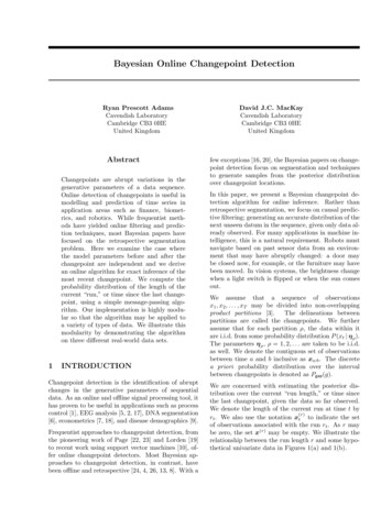
Figure 3: The top plot shows daily returns on the Dow Jones Industrial Average, with an overlaid plot of thepredictive volatility. The bottom plot shows the posterior probability of the current run length P (rt x1:t ) ateach time step, using a logarithmic color scale. Darker pixels indicate higher probability. The time axis is inbusiness days, as this is market data. Three events are marked: the conviction of G. Gordon Liddy and JamesW. McCord, Jr. on January 30, 1973; the beginning of the OPEC embargo against the United States on October19, 1973; and the resignation of President Nixon on August 9, 1974.(where pclose is the daily closing price) with a zeromean Gaussian distribution and piecewise-constantvariance. Hsu [14] performed a similar analysis on asubset of these data, using frequentist techniques andweekly returns.We used a gamma prior on the inverse variance, witha 1 and b 10 4 . The exponential prior on changepoint interval had rate λgap 250. In Figure 3, thetop plot shows the daily returns with the predictivestandard deviation overlaid. The bottom plot showsthe posterior probability of the current run length,P (rt x1:t ). Three events are marked on the plot:the conviction of Nixon re-election officials G. GordonLiddy and James W. McCord, Jr., the beginning ofthe oil embargo against the United States by the Organization of Petroleum Exporting Countries (OPEC),and the resignation of President Nixon.3.3COAL MINE DISASTER DATAThese data from Jarrett [15]
point detection focus on segmentation and techniques to generate samples from the posterior distribution over changepoint locations. In this paper, we present a Bayesian changepoint de-tection algorithm for online inference. Rather than retrospective segmentation, we focus on causal predic-tivefiltering; generatinganaccurate distribution ofthe next unseen datum in the sequence, given only .