WIXLIB

Cluster Analysis With SPSSI have never had research data for which cluster analysis was a technique I thoughtappropriate for analyzing the data, but just for fun I have played around with cluster analysis. Icreated a data file where the cases were faculty in the Department of Psychology at East CarolinaUniversity in the month of November, 2005. The variables are: Name -- Although faculty salaries are public information under North Carolina state law, Ithough it best to assign each case a fictitious name. Salary – annual salary in dollars, from the university report available in OneStop. FTE – Full time equivalent work load for the faculty member. Rank – where 1 adjunct, 2 visiting, 3 assistant, 4 associate, 5 professor Articles – number of published scholarly articles, excluding things like comments innewsletters, abstracts in proceedings, and the like. The primary source for these data was thefaculty member’s online vita. When that was not available, the data in the University’sAcademic Publications Database was used, after eliminating duplicate entries. Experience – Number of years working as a full time faculty member in a Department ofPsychology. If the faculty member did not have employment information on his or her webpage, then other online sources were used – for example, from the publications database Icould estimate the year of first employment as being the year of first publication. In the data file but not used in the cluster analysis are alsoArticlesAPD – number of published articles as listed in the university’s Academic PublicationsDatabase. There were a lot of errors in this database, but I tried to correct them (for example,by adjusting for duplicate entries).Sex – I inferred biological sex from physical appearance.Conducting the AnalysisStart by bringing ClusterAnonFaculty.savinto SPSS. Now click Analyze, Classify,Hierarchical Cluster. Identify Name as thevariable by which to label cases and Salary, FTE,Rank, Articles, and Experience as the variables.Indicate that you want to cluster cases ratherthan variables and want to display both statisticsand plots.You may want to open the output in a newtab while you are reading this document. Parts ofthe output have been inserted into this document.Click Statistics and indicate that you want to see an Agglomeration schedule with 2, 3, 4, and 5cluster solutions. Click Continue. Click Plots and indicate that you want a Dendogram and avertical Icicle plot with 2, 3, and 4 cluster solutions. Click Continue.ClusterAnalysis-SPSS

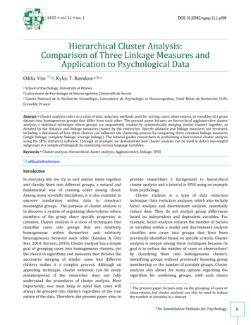
2Click Method and indicate that you want to use the Between-groups linkage method ofclustering, squared Euclidian distances, and variables standardized to z scores (so each variablecontributes equally). Click Continue. Click Save and indicate that you want to save, for eachcase, the cluster to which the case is assigned for 2, 3, and 4 cluster solutions. Click Continue,OK.SPSS starts by standardizing all of the variables to mean 0, variance 1. This results in all thevariables being on the same scale and being equally weighted.

3In the first step SPSS computes for each pair of cases the squared Euclidian distance2vbetween the cases. This is quite simply Xi Yi , the sum across variables (from i 1 to v) ofi 1the squared difference between the score on variable i for the one case (Xi) and the score onvariable i for the other case (Yi). The two cases which are separated by the smallest Euclidiandistance are identified and then classified together into the first cluster. At this point there is onecluster with two cases in it.Next SPSS re-computes the squared Euclidian distances between each entity (case or cluster)and each other entity. When one or both of the compared entities is a cluster, SPSS computesthe averaged squared Euclidian distance between members of the one entity and members of theother entity. The two entities with the smallest squared Euclidian distance are classified together.SPSS then re-computes the squared Euclidian distances between each entity and each otherentity and the two with the smallest squared Euclidian distance are classified together. Thiscontinues until all of the cases have been clustered into one big cluster.Look at the Agglomeration Schedule. On the first step SPSS clustered case 32 with 33. Thesquared Euclidian distance between these two cases is 0.000. At stages 2-4 SPSS creates threemore clusters, each containing two cases. At stage 5 SPSS adds case 39 to the cluster thatalready contains cases 37 and 38. By the 43rd stage all cases have been clustered into oneentity.Agglomeration ScheduleStageCluster Combined Coefficients Stage Cluster First Appears Next StageCluster 1 Cluster 2Cluster 1Cluster 2Cluster 1Cluster 1689.1430025

00Look at the Vertical Icicle. For the two cluster solution you can see that one cluster consists often cases(Boris through Willy, followed by a white column). These were our adjunct (part-time)faculty (excepting one) and the second cluster consists of everybody else.For the three cluster solution you can see that the cluster of adjunct faculty remains intact butthe other cluster is split into two. Deanna through Mickey were our junior faculty and Lawrencethrough Rosalyn our senior facultyFor the four cluster solution you can see that one case (Lawrence) forms a cluster of his own.

5Look at the Dendogram. It displays essentially the same information that is found in theagglomeration schedule but in graphic form.Look back at the data sheet. You will find three new variables. CLU2 1 is cluster membershipfor the two cluster solution, CLU3 1 for the three cluster solution, and CLU4 1 for the four clustersolution. Remove the variable labels and then label the values for CLU2 1

6and CLU3 1.Comparing the ClustersThe two group solution: Adjuncts vs others. Let us see how the two clusters in the twocluster solution differ from one another on the variables that were used to cluster them.The output shows that the cluster “Adjuncts” has lower mean salary, FTE, ranks, publishedarticles, and years experience.

7SalaryFTERankArticlesExperienceCLU2 1NMean Std. DeviationOthers34 60085 18665.11397Adjuncts 10 5956Others34 1.0000Adjuncts 10 .3750Others34 3.53Adjuncts 10Others34 14.91Adjuncts .904.77134 12.791.335Adjuncts 104.7010.688t-test for Equality of MeanstSalaryFTERankArticlesExperienceEqual variances assumed9.079dfSig. (2-tailed)42.000Equal variances not assumed 16.557 35.662.000Equal variances assumed42.000Equal variances not assumed 15.000 9.000.000Equal variances assumed42.000Equal variances not assumed 13.001 33.000.000Equal variances assumed42.019Equal variances not assumed 4.050 41.990.000Equal variances assumed42.051Equal variances not assumed 2.076 15.477.05528.4846.9922.4402.009The three cluster solution: Senior faculty, adjuncts, others. Now compare the threeclusters from the three cluster solution. Use One-Way ANOVA.

8ANOVASum of Squares dfBetween Groups 28416521260.677SalaryWithin GroupsTotalArticles3.018Within Groups.0043.175 43236.155Within Groups19.600 41.478Total91.909 43Between Groups5892.27622946.138Within Groups4647.633 41113.3573285.25121642.6252488.658 4160.6995773.909 43NMeanStd. DeviationSenior Faculty 10 80277.408018259.10829Others24 Senior Faculty 13176Senior Faculty 104.80.422Others243.00.885Adjuncts101.00.000Senior Faculty enior Faculty 1026.805.534246.967.178104.7010.688Experience OthersAdjuncts75.629 .00025.990 .00010539.909 43TotalArticles1.509 396.023 .00072.309Between GroupsRank2Between GroupsExperience Within GroupsFTE140500896.532.156 41TotalSalarySig.34177058018.482 43TotalRankF2 14208260630.339 101.126 .0005760536757.805 41Between GroupsFTEMean Square27.062 .000

9Predicting Salary from FTE, Rank, Publications, and ExperienceNow, just for fun, let us try a little multiple regression. We want to see how faculty salaries arerelated to FTEs, rank, number of published articles, and years of experience.Ask for part and partial correlations and for Casewise diagnostics for All cases.The output shows that each of our predictors is has a medium to large positive zero-ordercorrelation with salary, but only FTE and rank have significant partial effects. In the Casewise

10Diagnostic table you are given for each case the standardized residual (I think that any whoseabsolute value exceeds 1 is worthy of inspection by the persons who set faculty salaries), theactual salary, the salary predicted by the model, and the difference, in , between actual salaryand predicted salary.If you split the file by sex and repeat the regression analysis you will see some interestingdifferences between the model for women and the model for men. The partial effect of rank ismuch greater for women than for men. For men the partial effect of articles is positive andsignificant, but for women it is negative. That is, among our female faculty, the partial effect ofpublication is to lower one’s salary.Clustering VariablesCluster analysis can be used to cluster variables instead of cases. In this case the goal issimilar to that in factor analysis – to get groups of variables that are similar to one another. Again,I have yet to use this technique in my research, but it does seem interesting.We shall use the same data earlierused for principal components and factoranalysis, FactBeer.sav. Start out byclicking Analyze, Classify, HierarchicalCluster. Scoot into the variables box thesame seven variables we used in thecomponents and factors analysis. Under“Cluster” select “Variables.”Select Statistics and Plots as shown below.

11Click “Method” andI have saved, annotated, and placed online the statistical output from the analysis. You maywish to look at it while reading through the remainder of this document.Look at the proximity matrix. It is simply the intercorrelation matrix. We start out with eachvariable being an element of its own. Our first step is to combine the two elements that areclosest – that is, the two variables that are most well correlated. As you can from the proximitymatrix, that is color and aroma (r .909). Now we have six elements – one cluster and fivevariables not yet clustered.In Stage 2, we cluster the two closest of the six remaining elements. That is size and alcohol(r .904). Look at the agglomeration schedule. As you can see, the first stage involvedclustering variables 5 and 6 (color and aroma), and the second stage involved clustering variables2 and 3 (size and alcohol).

12In Stage 3, variable 7 (taste) is added to the cluster that already contains variables 5 (color)and 6 (aroma).In Stage 4, variable 1 (cost) is added to the cluster that already contains variables 2 (size)and 3 (alcohol). We now have three elements – two clusters, each with three variables, and onevariable not yet clustered.In Stage 5, the two clusters are combined, but note that they are not very similar, the similaritycoefficient being only .038. At this point we have two elements, the reputation variable all aloneand the six remaining variables clumped into one cluster.The remaining plots show pretty much the same as what I have illustrated with the proximitymatrix and agglomeration schedule, but in what might be more easily digested format.I prefer the three cluster solution here. Do notice that reputation is not clustered until the verylast step, as it was negatively correlated with the remaining variables. Recall that in thecomponents and factor analyses it did load (negatively) on the two factors (quality and cheapdrunk).Karl L. WuenschEast Carolina UniversityDepartment of PsychologyGreenville, NC 27858-435317-January-2016More SPSS LessonsMore Lessons on Statistics

Cluster Analysis With SPSS I have never had research data for which cluster analysis was a technique I thought appropriate for analyzing the data, but just for fun I have played around with cluster analysis. I created a data file where the cases were faculty in the Department of Psychology at East CarolinaFile Size: 685KBPage Count: 12Explore furtherCluster analysis with SPSS: Hierarchical Cluster Analysiswww.fmi-plovdiv.orgSPSS Tutorial - Multivariate Solutionswww.mvsolution.comHierarchical Cluster Analysis - PSS Factor Analysis - Absolute Beginners Tutorialwww.spss-tutorials.comCluster Analysis - IBM SPSS Statistics Guides: Straight .norusis.comRecommended to