WIXLIB

5][7-8]. To do so, we first construct the network topologyfrom domain knowledge and subject matter experts [9-12],similar to the fundamental analysis process. Then, weillustrate the technical analysis aspect in which theconditional probabilities between children and parent nodesof the directed arcs in the network are learned statisticallyfrom the historical data.There are many factors affecting S&P market dynamics.Some of the most obvious examples include interest rate(LIBOR), consumer price index (CPI), unemployment rate(UR), money supply (MS), housing start (HS), and impliedvolatility index (VIX). Note that interest rate is animportant driver of the nation’s economy. Stock markettends to go higher when the interest rate is low which alsomakes other alternative investment such as fixed incometreasuries less attractive. CPI measures the inflation level ofthe consumer price and is highly relevant to the overalleconomics and equity market.Unemployment rate is also an important factor that couldaffect the market direction. A high unemployment ratemight be bad for the market depending on other factors suchas government momentary policy. In addition, moneysupply and housing start may have some impact on themarket direction as well. Finally the implied volatilityindex (VIX, also called the fear and greed index) measuresthe S&P volatility based on the S&P one-month options andmight be a good indicator of market direction. Highvolatility implies a potential down trend and vice versa.Taking into account of aforementioned key economicfactors, we construct an exemplary Bayesian network tomodel the S&P dynamics, as shown in Figure 1. This modelhas been obtained by working with subject matter expertsand validated by historical data. Among the factorsmentioned earlier, some of them (money supply andhousing start) are eliminated due to their weak correlationsto the S&P future directions. In the network, each node ismodeled as a binary random variable with two state values:“up” or “down”. Note that in Figure 1, SP2 indicates thepotential future S&P state (“up” or “down”) for the nexttrading period and SP1 represents the S&P state in thecurrent trading period. The remaining variables in thenetwork represent their corresponding states in the currentperiod. For example, an “up” state for VIX (VX1) indicatesthe implied volatility has gone up in the current time period.The purpose of the BN model is to predict S&P marketdirection for the next trading period in order to facilitatetrading decision or risk management. The networkparameters (conditional probabilities of a child node givenits parents) are learned from the historical data [15]. Thehistorical data is organized in a sliding widow manner sothat a series of past data can be used to train the model forpredicting the probability of the market trend at the nexttime period.1924Specifically, we collected the historical data from 1990 to2014, where the S&P and VIX data are obtained from theyahoo finance web site and the rest are downloaded fromFederal Reserve economic data repository [16].Specifically, we set the trading cycle to be one month andthe training window size to be 180 months. In other words,we use the historical data from the past 180 months to trainthe model and apply it to predict the market direction for thenext trading month. We repeat the prediction process from2005 to 2014 for 120 trading months. An example set ofconditional probability tables (CPT) in the network learnedfrom the historical data is shown in Table 1.Figure 1. A Bayesian Network for S&P Dynamic ModelTable 1. An example set of CPTs leanred from historical dataSP2 ��“down”“down”SP2 “down”0.39VX1 wn”VX1 “down”0.580.50SP1 “up”0.310.840.260.88SP1 “down”0.690.160.740.11SP2“up”“down”LB1 “up”0.420.40LB1 “down”0.580.60SP2“up”“down”UR1 “up”0.310.40UR1 down”UR1“up”“down”“up”“down”CP1 “up”0.790.760.680.95CP1 “down”0.210.240.320.05

2.2c S0 N(d1 ) ! K e!rT N(d2 )Trading S&P Futures and OptionsS&P futures and their options are traded in several financialmarkets, such as the Chicago Mercantile Exchange (CME)[17] and the CME electronic GLOBEX platform [18]. Thereare several common trading practices on the markets [21], asquoted below from Wikipedia. Long: a long position is to buy or own a underlyingentity (e.g., asset, index, or interest rate futures); Short: a short position is to sell or owe; Put: a put option gives the owner of the put, the right,but not the obligation, to sell an asset (the underlying)at a specific price (the strike), by a pre-determined date(the expiration or maturity date) to a given party (theseller of the put). Put options are most commonly usedin the stock market to protect against the decline of astock price below a specific price. Call: a call option gives the buyer of the call, the right,but not the obligation, to buy an agreed quantity of theunderlying from the seller (or “writer”) of the calloption before a certain time (the expiration date) at acertain strike price.S&P futures is one of the most liquid futures markets inthe world. One can long or short the futures contracts aslong as there is a counter party who is willing to take theopposite side. Similarly, the S&P futures options market isextremely liquid and popular. One could long or short theput or call options depending on the goals of the tradingstrategies.By writing (selling) the put options when the market isexpected to go higher would result in the options expiringworthlessly and therefore the seller could keep the collectedpremium. Similarly, the seller could keep the premiumcollected by writing the call options if the market does notgo up. However, while the potential loss of buying optionsis limited by the premium paid, shorting options could bevery risky because the loss is only limited by the marketactions. For example, shorting a call option while themarket continues going up could result in a severe loss.2.3Options Pricing ModelTo derive the fair option price, a common practice is toassume that the underlying asset follows a geometricBrownian motion (GBM) model with constant drift andvolatility, described by the following stochastic differentialequation:dS µ S dt ! S dW(1)where S is the asset price, µ is the drift parameter, ! is thevolatility, and W is a wiener process or Brownian motion.With the assumed model, a closed-form options pricingmodel has been developed [19-20], as follows:1925(2)p K e!rT N(!d2 ) ! S0 N(!d1 )whered1 ln(S0 / K ) (r ! 2 / 2)T! Tln(S / K ) (r ! ! 2 / 2)T(3)0 d1 ! ! T! TIn eqn. (2), c is the price of a call option, p is for put option,S0 is the current asset price, K is the strike price, T is thematurity (expiration) time, and ! is the asset volatility. Thispopular Back-Scholes-Merton (BSM) option pricing modelhad revolutionized the derivative industry for the lastseveral decades.d2 Note that the value of an option consists of both timevalue and intrinsic value. While the intrinsic value dependson the relative strike price to the asset value, the time valuealways reduces to zero at the expiration. As mentionedearlier, an important assumption behind the derivation ofthe BSM pricing model is that the price of the underlyingasset follows a GBM model with constant drift andvolatility.However, since the stock crash of October 1987, thevolatility of stock index options implied by the marketprices has been observed to be “skewed” in the sense thatthe volatility became a function of strike and expirationinstead of remaining a constant. This phenomenon referredto as the “volatility smile” has since spread to other markets[21]. Because the original BSM model can no longeraccount for the smile, investors have to use more complexmodels to value and hedge their options. In this paper, forthe purpose of evaluating the trading performance, we willemulate the option prices subject to the smile phenomenonby utilizing the historical implied volatility index (VIX)data and approximate the volatility smile as a quadraticfunction of moneyness1 [22].2.4Trading ProcessAs mentioned earlier, the target node (SP2) in theBayesian network shown in Figure 1 represents the one-stepprediction of the S&P market in the next trading cycle. Weuse a monthly cycle to synthesize the trading process. Atthe beginning of each month, we simulate the trading on theS&P futures and options markets based on the strategiesderived from the BN model predictions. We use historicalend-of-the-day S&P settlement prices and the optionspricing model (Section 2.3) to emulate the filled-prices ofthe transactions. We assume no transaction cost and noslippage.1Moneyness is the relative position of the current price of anunderlying asset with respect to the strike price of a derivative.

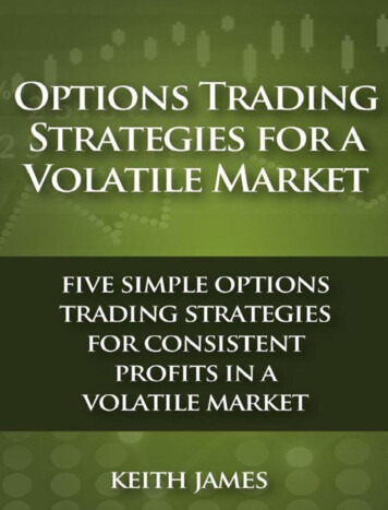
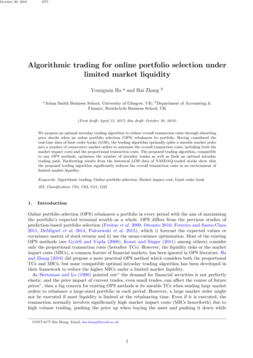
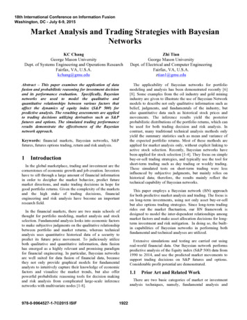
3Test and Simulation3.3We apply two trading strategies based on the BNprediction. The first strategy is “Long and Short” where weeither long the S&P index futures if the prediction is “up” orshort the futures if the prediction is “down”. The secondstrategy is “Options Writing” where we either short theS&P futures put options when the predicted trend isexpected to be up or short the call options when the trend isexpected to be down.We compare the tradingperformances to the naïve buy-and-hold strategy.3.1Long and Short StrategyIn the “Long and Short” (LS) strategy we either long theS&P if the prediction is “up” (posterior probability of SP2 is“up” is greater than 0.5) or short the S&P if the prediction is“down” (posterior probability of SP2 is “down” is greaterthan 0.5). We apply a monthly trading cycle to test thestrategy. On the first trading day of each month, if thepredicted trend is up for the coming month, 100% of theequity will be committed to a long position of the S&Pfutures for the entire month. Similarly, 100% equity will becommitted to a short S&P futures position for the entiremonth if the prediction is down.3.2Options Writing StrategyWith “Options Writing” (OW) strategy, we either shortthe S&P put options when the trend is expected to be up(posterior probability of SP2 is “up” is greater than 0.5) orshort the call options when the trend is expected to be down(posterior probability of SP2 is “down” is greater than 0.5).We also apply a monthly trading cycle to be consistent withthe monthly expiration options. Specifically, if the marketis predicted to be up, we will short the at-the-money2(ATM) S&P put options expiring in the coming month; andif the market prediction is down, we will short thecorresponding S&P ATM call options. We will keep theoptions until expiration before repeating the same process inthe next trading cycle.Note that the options could expire out of the money3(OTM), and therefore become worthless. In that case, thepremium collected by the seller becomes the profit and thepositions will be closed automatically by the exchange. Onthe other hand, if the options expire in the money (ITM), theoptions will have to be settled in cash in the sense that thesellers have to pay the market price to “buy” back theoptions they sold. In that case, if the market price is higherthan the premium collected, the seller will incur a loss.Simulated TradingFigure 2 shows the historical data of the relevant factorsin the BN model. Since there are only limited historicaloptions prices with specific strikes and expirations availablein the public domain, we simulate the options filled-pricesbased on the model described earlier. Specifically, optionsprices are obtained by utilizing the BSM model given theS&P price, risk-free interest rate, volatility, and anexpiration date of 4 trading weeks after writing the options.The S&P prices are based on historical data and served asthe ATM strike prices. Risk-free interest is based onhistorical 3-month LIBOR data and volatility is based onthe historical implied volatility index (VIX). However, asmentioned earlier, it is well known that true volatility is nota constant but a function of strike and expiration (volatilitysmile and surface). To obtain a more realistic options price,we develop a smile model and adjust the option priceaccordingly as described in Section 2.3. The results havebeen validated against the available market data and provedto be reasonably accurate.3.4Performance ResultsFigure 3 summarizes the performance of the LS strategy.As shown in the figure, the strategy longs the market mostof the time, while shorts the market only about 10% of thetime based on the assessed probabilities obtained by theBayesian network model. The performance of this dynamictrading strategy is significantly better than the buy-and-holdapproach while with smaller risk/volatility.Figure 4 shows the performance of the OW strategy. Asshown in the figure, while the rate of return is lower thanthat of the LS strategy over the 10 years period, thepercentage of positive return is much higher (75% vs. 63%).The rate of return of this dynamic trading strategy is alsomuch higher then the buy-and-hold approach while withsmaller risk/volatility. Note that one could easily employleverage in options trading. Typically, the trader is allowedto have up to 10 to 1 leverage by the exchange. Forexample, with a 2 to 1 leverage (OW-II, selling twice asmany as options contracts per capital) and a 4 to 1 leverage(OW-IV), the performances are shown in Figures 5 and 6,respectively. The results show that with higher leverage, thereturns are much better while the risk is also increased. Thestrategy is clearly very effective and flexible. Depending onthe risk aptitude of the investor, one could conceivablyadjust the leverage level to meet a range of desirableinvestment goals with different risk-reward trade-offs.Table 2 summarizes the trading results. In the table, twoadditional performance metrics, maximum drawdown andSharpe ratio, are given for comparison. Specifically,drawdown is defined as the peak-to-trough decline during aspecific period of an investment. The Sharpe ratio is ameasure for calculating risk-adjusted return. It is the averagereturn earned in excess of the risk-free rate over the returnvolatility (standard deviation). It can be seen from the table2When the option strike price is equal to the current price of theunderlying asset.3The strike of a call option is above the market price or the strikeof a put option is below the market price of the underlying asset.1926

that LS and OW perform much better than the naïve buyand-hold policy. The BN-based strategies not only offerhigher returns over the 10-year period, but also exhibitsmaller drawdowns and volatilities. Furthermore, byemploying leveraged options writing strategies, theperformance can be adapted for different risk/reward levels.For example, an aggressive investor might decide to employa higher leverage ratio than a conservative one.Table 2. Performance ComparisonBuy-HoldLS (BN)OW-I (BN)OW-II (BN)OW-IV (BN)4PositiveReturn62.2%63.0%74.8%74.8%74.8%Rate of Return(10 860.89ConclusionWe have developed a data fusion approach usingBayesian networks for predicting market directions tosupport investment and trading decisions. The Bayesiannetwork is constructed from both historical data and domainknowledge of several relevant financial factors. Theresulting model is applied to predict the S&P direction forthe next trading cycle. Several trading strategies areimplemented based on the market predictions. The resultsof the simulated trading using these strategies over a 10year period show considerable potential equity gains. TheBN-based strategies significantly outperform the naïve buyand-hold policy, which demonstrate the potential andeffectiveness of the BN approach.Figure 2. Historical Data of Relevant FactorsReferences[1] Yi Zuo and Eisuke Kita, “Up/Down Analysis of StockIndex by using Bayesian Network,” EngineeringManagement Research, Vol. 1, No. 2, 2012.[2] Yi Zuo and Eisuke Kita, “Stock Price Forecast usingBayesian Network,” Expert Systems with Applications,Elsvier, Vol. 39, pp. 6729-6737, 2012.[3] Jangmin O., Jae Won Lee, SB Lark, and BT Zhang,“Stock trading by Modeling Price Trend with DynamicBayesian Networks,” IDEAL, pp. 794-799, 2004.[4] N. G. Polson and Bernard V. Tew, “Bayesian PortfolioSelection: An Empirical Analysis of the S&P 500 Index19070-1996,” ASA Journal of Business and EconomicStatistics, Vol. 18, No. 2, 2000.[5] John Geweke and Gianni Amisano, “Comparing andEvaluating Bayesian Predictive Distributions of AssetReturns,” European Central Bank Eurosystem, Workingpaper No. 969, 2008.1927Figure 3. Long and Short Trading Performance

Figure 4. Options Writing Strategy with No Leverage (OW-I)Figure 6. Options Writing with 4 to 1 Leverage (OW-IV)[6] Yi Zuo and Eisuke Kita, “Up/Down Analysis of StockIndex by using Bayesian Network,” EngineeringManagement Research, Vol. 1, No. 2, 2012.[7] Yi Zuo and Eisuke Kita, “Stock Price Forecast usingBayesian Network,” Expert Systems with Applications,Elsvier, Vol. 39, pp. 6729-6737, 2012.[8] Jangmin O., Jae Won Lee, SB Lark, and BT Zhang,“Stock trading by Modeling Price Trend with DynamicBayesian Networks,” IDEAL, pp. 794-799, 2004.[9] N. G. Polson and Bernard V. Tew, “Bayesian PortfolioSelection: An Empirical Analysis of the S&P 500 Index19070-1996,” ASA Journal of Business and EconomicStatistics, Vol. 18, No. 2, 2000.[10] John Geweke and Gianni Amisano, “Comparing andEvaluating Bayesian Predictive Distributions of AssetReturns,” European Central Bank Eurosystem, Workingpaper No. 969, 2008.[11] Riza Demirer Ronald R. Mau, and Catherine Shenoy,“Bayesian Networks: A Decision tool to Improve PortfolioRisk Analysis,” Journal of Applied Finance (Winter 2006),106–119.Figure 5. Options Writing with 2 to 1 Leverage (OW-II)1928

[12] Daniel Anderson, “Stock Investing using HUGINSoftware – An Easy Way to use Quantitative webdocs/CaseStories/WP stock picking.pdf[13] Catherine Shenoy and Prakash P. Shenoy, “BayesianNetwork Models of Portfolio Risk and Return,” in Y. S.Abu-Mostafa, B. LeBaron, A W. Lo, and A. S. Weigand(eds.), Computational Finance 1999, pp. 87--106, The MITPress, Cambridge, MA.[14] Nathan Taulbee, “Influences on the Stock Market:Examination of the Effect of Economic Variables on S&P500,” The Park Place Economist: Vol. 9, No. 1, iss1/20[15] Charles Cao and Jing-Zhi Hiang, “Determinants ofS&P Index Option Returns,” Rev Deriv Res, 10:1–38, 2007.[16] Mark J. Flannery and Aris A. Protopapadakis,“Macroeconomic Factors do Influence Aggregate StockReturns,” The Review of Financial Studies, Vol. 15, No. 3,pp. 751-782, 2002.[17] Martin Sirucek, “Macroeconomic Variables and StockMarket: US Review,” MPRA Paper No. 39094, May 2012.http://mpra.ub.uni-muenchen.de/39094/[18] Ioannis Karatzas, Steve Shreve, Methods ofMathematical Finance. Secaucus, NJ, USA: SpringerVerlag New York, Incorporated, 1998.[19] Daphne Koller and Nir Friedman, ProbabilisticGraphical Models, MIT Press, 2009.[20] Borgelt C, Kruse R, and Steinbrecher M, GraphicalModels: Representations for Learning, Reasoning and DataMining, Wiley, 2nd edition, 2009.[21] Federal Reserve Economic Data, St. Louis FRED,http://research.stlouisfed.org/fred2/[22] -index/sandp-500 c

Market Analysis and Trading Strategies with Bayesian Networks KC Chang . futures, futures options trading, return and risk analysis. 1 Introduction In the global marketplace, trading and investment are the . modeled as a binary random variable with two state values: