Transcription
1Microsoft Excel 2010 TutorialExcel is a spreadsheet program in the Microsoft Office system. You can use Excel to create and format workbooks (a collection ofspreadsheets) in order to analyze data and make more informed business decisions. Specifically, you can use Excel to track data, buildmodels for analyzing data, write formulas to perform calculations on that data, pivot the data in numerous ways, and present data in a varietyof professional looking charts.The RibbonUnderstanding the Ribbon is a great way to help understand the changes between Microsoft 2003 to Microsoft 2010. The ribbon holds all ofthe information in previous versions of Microsoft Office in a more visual stream line manner through a series of tabs that include an immensevariety of program features.Home TabThis is the most used tab; it incorporates all text and cell formatting features such as font and paragraph changes. The Home Tab alsoincludes basic spreadsheet formatting elements such as text wrap, merging cells and cell style.Insert TabThis tab allows you to insert a variety of items into a document from pictures, clip art, and headers and footers.Page Layout TabThis tab has commands to adjust page such as margins, orientation and themes.Created By: Amy BeaucheminSource: office.microsoft.com1/13/11
2Formulas TabThis tab has commands to use when creating Formulas. This tab holds an immense function library which can assist when creating anyformula or function in your spreadsheet.Data TabThis tab allows you to modifying worksheets with large amounts of data by sorting and filtering as well as analyzing and grouping data.Review TabThis tab allows you to correct spelling and grammar issues as well as set up security protections. It also provides the track changes andnotes feature providing the ability to make notes and changes someone’s document.View TabThis tab allows you to change the view of your document including freezing or splitting panes, viewing gridlines and hide cells.Created By: Amy BeaucheminSource: office.microsoft.com1/13/11
3Getting StartedNow that you have an understanding of where things are located, let’s look at the steps needed to createan Excel document.Opening OutlookYou may have a shortcut to Word on your desktop, if so double click the icon and Word will open. If notfollow the steps below:1. Click on the Start button2. Highlight Programs3. Highlight Microsoft Office4. Click on Microsoft Excel 2010Create a New Workbook1. Click the File tab and then click New.2. Under Available Templates, double click Blank Workbook or Click Create.Find and Apply TemplateExcel 2010 allows you to apply built-in templates and to search from a variety of templates onOffice.com. To find a template in Excel 2010, do the following:1. On the File tab, click New.2. Under Available Templates, do one of the following:a. To reuse a template that you’ve recently used, click Recent Templates, click the templatethat you want, and then click Create.b. To use your own template that you already have installed, click My Templates, select thetemplate that you want, and then click OK.c. To find a template on Office.com, under Office.com Templates, click a template category,select the template that you want, and then click Download to download the template fromOffice.com to your computer.3. Once you click on the template you like it will open on your screen as a new document.Enter Data in a Worksheet1. Click the cell where you want to enter data.2. Type the data in the cell.3. Press enter or tab to move to the next cell.Created By: Amy BeaucheminSource: office.microsoft.com1/13/11
4Select Cells or RangesIn order to complete more advanced processes in Excel you need to be able to highlight or select cells,rows and columns. There are a variety of way to do this, see the table below to understand the options.To selectA single cellA range of cellsA large range of cellsDo thisClick the cell, or press the arrow keys to move to the cell.Click the first cell in the range, and then drag to the last cell, or hold downSHIFT while you press the arrow keys to extend the selection.Click the first cell in the range, and then hold down SHIFT while you click thelast cell in the range. You can scroll to make the last cell visible.All cells on a worksheetClick the Select All button or press CTRL A.Nonadjacent cells or cellrangesAn entire row or columnSelect the first cell or range of cells, and then hold down CTRL while you selectthe other cells or ranges.NOTE: You cannot cancel the selection of a cell or range of cells in anonadjacent selection without canceling the entire selection.Click the row or column heading.Row headingColumn headingAdjacent rows or columns Drag across the row or column headings. Or select the first row or column;then hold down SHIFT while you select the last row or column.Nonadjacent rows orClick the column or row heading of the first row or column in your selection;columnsthen hold down CTRL while you click the column or row headings of other rowsor columns that you want to add to the selection.Cells to the last used cell Select the first cell, and then press CTRL SHIFT END to extend the selectionon the worksheet (lower- of cells to the last used cell on the worksheet (lower-right corner).right corner)Cells to the beginning of theSelect the first cell, and then press CTRL SHIFT HOME to extend theworksheetselection of cells to the beginning of the worksheet.NOTE: To cancel a selection of cells, click any cell on the worksheet. This is not applicable to cells withformulas in it.Modifying SpreadsheetsIn order to create an understandable and professional document you will need to make adjustments tothe cells, rows, columns and text. Use the following processes to assist when creating a spreadsheet.Cut, Copy, and Paste DataYou can use the Cut, Copy, and Paste commands in Microsoft Office Excel to move or copy entire cellsor their contents. NOTE: Excel displays an animated moving border around cells that have been cut orcopied. To cancel a moving border, press ESC.Created By: Amy BeaucheminSource: office.microsoft.com1/13/11
5Move/Copy CellsWhen you move or copy a cell, Excel moves or copies the entire cell,including formulas and their resulting values, cell formats, and comments.1. Select the cells that you want to move or copy.2. On the Home tab, in the Clipboard group, do one of the following:a. To move cells, click Cut.b. To copy cells, click Copy.3. Click in the center of the cell you would like to Paste the information too.4. On the Home tab, in the Clipboard group, click Paste.NOTES: Excel replaces existing data in the paste area when you cut and paste cells to move them.When you copy cells, cell references are automatically adjusted. If the selected copy or paste areaincludes hidden cells, Excel also copies the hidden cells. You may need to temporarily unhide cells thatyou don't want to include when you copy information.Move/Copy Cells with Mouse1. Select the cells or a range of cells that you want to move or copy.2. To move a cell or range of cells, point to the border of the selection. When the pointer becomes amove pointer, drag the cell or range of cells to another location.Column Width and Row HeightOn a worksheet, you can specify a column width of 0 to 255 and a row height of 0 to 409. This valuerepresents the number of characters that can be displayed in a cell that is formatted with the standardfont. The default column width is 8.43 characters and the default rowheight is 12.75 points. If a column/row has a width of 0, it is hidden.Set Column/Row Width/Height1. Select the column(s) or row(s) that you want to change.2. On the Home tab, in the Cells group, click Format.3. Under Cell Size, click Column Width or Row Height.4. A Column Width or Row Height box will appear.5. In the Column Width or Row Height box, type the value that youwant your column or row to be.Automatically Fit Column/Row Contents1. Click the Select All button2. Double-click any boundary between two column/rowheadings.3. All Columns/Rows in the entire worksheet will bechanged to the new sizeNOTE: At times, a cell might display #####. This can occur when the cell contains a number or a datethat exceeds the width of the cell so it cannot display all the characters that its format requires. To seethe entire contents of the cell with its current format, you must increase the width of the column.Created By: Amy BeaucheminSource: office.microsoft.com1/13/11
6Set Column/Row Width/Height with MouseTo change the width of one column/row1. Place you cursor on the line between two rows or columns.2. A symbol that looks like a lower case t with arrows on the horizontalline will appear3. Drag the boundary on the right side of the column/row heading until thecolumn/row is the width that you want.To change the width of multiple columns/rows1. Select the columns/rows that you want to change2. Drag a boundary to the right of a selected column/row heading.3. All selected columns/rows will become a different size.To change the width of columns/rows to fit the contents in the cells1. Select the column(s) or row(s) that you want to change2. Double-click the boundary to the right of a selected column/row heading.3. The Column/Row will automatically be size to the length/height of the longest/tallest text.Merge or Split CellsWhen you merge two or more adjacent horizontal or vertical cells the cells become one larger cell that isdisplayed across multiple columns or rows. When you merge multiple cells, the contents of only one cellappear in the merged cell.Merge and Center Cells1. Select two or more adjacent cells that you want to merge.2. On the Home tab, in the Alignment group, click Merge and Center.3. The cells will be merged in a row or column, and the cell contents will be centered in the merged cell.Merge CellsTo merge cells only, click the arrow next to Merge and Center, and then clickMerge Across or Merge Cells.Split Cells1. Select the merged cell you want to split2. To split the merged cell, click Merge and Center. The cells will splitand the contents of the merged cell will appear in the upper-left cell of the range of split cells.Automatically Fill DataTo quickly fill in several types of data series, you can select cells and drag the fill handle. To usethe fill handle, you select the cells that you want to use as a basis for filling additional cells, and then dragthe fill handle across or down the cells that you want to fill.1. Select the cell that contains the formula that you want to be brought to other cells.2. Move your curser to the small black square in the lower-right corner of a selected cell also know asthe fill handle. Your pointer will change to a small black cross.3. Click and hold your mouse then drag the fill handle across the cells, horizontally to the right orvertically down, that you want to fill.4. The cells you want filled will have a gray looking border around them. Once you fill all of the cells letgo of your mouse and your cells will be populated.Created By: Amy BeaucheminSource: office.microsoft.com1/13/11
7Formatting SpreadsheetsTo further enhance your spreadsheet you can format a number of elements such as text, numbers,coloring, and table styles. Spreadsheets can become professional documents used for companymeetings or can even be published.Wrap TextYou can display multiple lines of text inside a cell by wrapping the text. Wrapping text in a cell does notaffect other cells.1. Click the cell in which you want to wrap the text.2. On the Home tab, in the Alignment group, click Wrap Text.3. The text in your cell will be wrapped.NOTE: If the text is a long word, the characters won't wrap (theword won't be split); instead, you can widen the column or decrease the font size to see all the text. If allthe text is not visible after you wrap the text, you might have to adjust the height of the row. On theHome tab, in the Cells group, click Format, and then under Cell Size click AutoFit RowFormat NumbersIn Excel, the format of a cell is separate from the data that is stored in the cell. This display differencecan have a significant effect when the data is numeric. For example, numbers in cells will default asrounded numbers, date and time may not appear as anticipated. After you type numbers in a cell, youcan change the format in which they are displayed to ensure the numbers in your spreadsheet aredisplayed as you intended.1. Click the cell(s) that contains the numbers that you want to format.2. On the Home tab, in the Number group, click the arrow next to theNumber Format box, and then click the formatthatyou want.If you are unable to format numbers in the detail you would like that you can clickon the More Number Formats at the bottom of the Number Format drop downlist.1.In the Category list, clickthe format that you want to use,and then adjust settings to theright of the Format Cells dialogbox. For example, if you’re usingthe Currency format, you canselect a different currencysymbol, show more or fewerdecimal places, or change theway negative numbers aredisplayed.Created By: Amy BeaucheminSource: office.microsoft.com1/13/11
8Cell BordersBy using predefined border styles, you can quickly add a border around cells or ranges of cells. Ifpredefined cell borders do not meet your needs, you can create a custom border.NOTE: Cell borders that you apply appear on printed pages. If you do not use cell borders but wantworksheet gridline borders for all cells to be visible on printed pages, you can display the gridlines.Apply Cell Borders1. On a worksheet, select the cell or range of cells that you want toadd a border to, change the border style on, or remove a borderfrom.2. Go to the Home tab, in the Font group3. Click the arrow next to Borders4. Click on the border style you would like5. The border will be applied to the cell or cell rangeNOTE: To apply a custom border style, click More Borders. In theFormat Cells dialog box, on the Border tab, under Line and Color,click the line style and color that you want.Remove Cell Borders1. Go to the Home tab, in the Font group2. Click the arrow next to Borders3. Click No Border.NOTES: The Borders button displays the most recently usedborder style. You can click the Borders button (not the arrow) toapply that style.Cell StylesYou can create a cell style thatincludes a custom border, colors andaccounting formatting.1. On the Home tab, in the Stylesgroup, click Cell Styles.2. Select the different cell styleoption you would like applied toyour spreadsheet.NOTE: If you would like to apply acell fill and a cell border, select thecell fill color first the ensure bothformats are applied.Created By: Amy BeaucheminSource: office.microsoft.com1/13/11
9Cell and Text ColoringYou can also modify a variety of cell and text colors manually.Cell Fill1. Select the cells that you want to apply or remove a fill color from.2. Go to the Home tab, in the Font group and select one of thefollowing options:a. To fill cells with a solid color, click the arrow next to FillColor, and then under Theme Colors or StandardColors, click the color that you want.b. To fill cells with a custom color, click the arrow next to FillColor, click More Colors, and then in the Colors dialogbox select the color that you want.c. To apply the most recently selected color, click Fill Color.NOTE: Microsoft Excel saves your 10 most recently selectedcustom colors. To quickly apply one of these colors, click the arrownext to Fill ColorRecent Colors., and then click the color that you want underRemove Cell Fill1. Select the cells that contain a fill color or fill pattern.2. On the Home tab, in the Font group, click the arrow next to FillColor, and then click No Fill.Text Color1. Select the cell, range of cells, text, or characters that you want to format with a different text color.2. On the Home tab, in the Font group and select one of the following options:a. To apply the most recently selected text color, click Font Color.b. To change the text color, click the arrow next to Font Color, and then under ThemeColors or Standard Colors, click the color that you want to use.Bold, Underline and Italics Text1. Select the cell, range of cells, or text.2. Go to the Home tab, in the Font group3. Click on the Bold (B) Italics (I) or Underline (U) commands.4. The selected command will be applied.Customize Worksheet Tab1. On the Sheet tab bar, right-click the sheet tab that you want to customize2. Click Rename to rename the sheet or Tab Color to select a tab color.3. Type in the name or select a color you would like for your spreadsheet.4. The information will be added to the tab at the bottom of the spreadsheet.Created By: Amy BeaucheminSource: office.microsoft.com1/13/11
10Formulas in ExcelFormulas are equations that perform calculations on values in your worksheet. A formula always startswith an equal sign ( ). An example of a simple is 5 2*3 that multiplies two numbers and then adds anumber to the result. Microsoft Office Excel follows the standard order of mathematical operations. In thepreceding example, the multiplication operation (2*3) is performed first, and then 5 is added to its result.You can also create a formula by using a function which is a prewritten formula that takes a value,performs an operation and returns a value. For example, the formulas SUM(A1:A2) and SUM(A1,A2)both use the SUM function to add the values in cells A1 and A2.Depending on the type of formula that you create, a formula can contain any or all of the following parts.Functions A function, such as PI() or SUM(), starts with an equalsign ( ).Cell references You can refer to data in worksheet cells by includingcell references in the formula. For example, the cell reference A2returns the value of that cell or uses that value in the calculation.Constants You can also enter constants, such as numbers (such as 2) or text values, directly into aformula.Operators Operators are the symbols that are used to specify the type of calculation that you want theformula to perform.EXAMPLEWHAT IT DOESCreate a Simple FormulasFORMULA1. Click the cell in which you want to enter the formula. 5 2Adds 5 and 22. Type (equal sign). 5-2Subtracts 2 from 53. Enter the formula by typing the constants and operators 5/2Divides 5 by 2that you want to use in the calculation. 5*2Multiplies 5 times 24. Press ENTER. 5 2Raises 5 to the 2nd powerCreate a Formula with Cell References1.2.3.4.5.6.The first cell reference is B3, the color is blue, and the cell rangehas a blue border with square corners.The second cell reference is C3, the color is green, and the cellrange has a green border with square corners.To create your formula:Click the cell in which you want to enter the formula.In the formula bar, at the top of the Excel window that you use,, type (equal sign).stClick on the 1 cell you want in the formula.Enter an Operator suchEXAMPLE WHAT IT DOESas , or *.FORMULAClick on the next cell you A1 A2Adds the values in cells A1 and A2want in the formula.Subtracts the value in cell A2 from the value in A1Continue steps 3 – 5 until A1-A2 A1/A2Divides the value in cell A1 by the value in A2the formula is complete A1*A2Multiplies the value in cell A1 times the value in A2Hit the ENTER key on A1 A2Raises the value in cell A1 to the exponential valueyour keyboard.specified in A2Created By: Amy BeaucheminSource: office.microsoft.com1/13/11
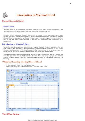
11Create a Formula with Function1. Click the cell in which you want to enter theformula.2. Click Insert Functionon the formula bar. Excel inserts the equal sign ( ) foryou.3. Select the function that you want to use.NOTE: If you're not sure which function to use,type a question that describes what you want todo in the Search for a function box (forexample, "add numbers" returns the SUMfunction), or browse from the categories in theOr Select a category box.4. Enter the arguments.5. After you complete the formula, press ENTER.Use Auto SumTo summarize values quickly, you can also use AutoSum.1. Select the cell where you would like your formulas solution to appear.2. Go to the Home tab, in the Editing group,3. Click AutoSum, to sum your numbers or click the arrow next to AutoSum toselect a function that you want to apply.Delete a FormulaWhen you delete a formula, the resulting values of the formula is also deleted. However, you can insteadremove the formula only and leave the resulting value of the formula displayed in the cell.To delete formulas along with their resulting values, do the following:1. Select the cell or range of cells that contains the formula.2. Press DELETE.To delete formulas without removing their resulting values, do thefollowing:1. Select the cell or range of cells that contains the formula.2. On the Home tab, in the Clipboard group, click Copy.3. On the Home tab, in the Clipboard group, click the arrow below PasteValues.Created By: Amy BeaucheminSource: office.microsoft.com, and then click Paste1/13/11
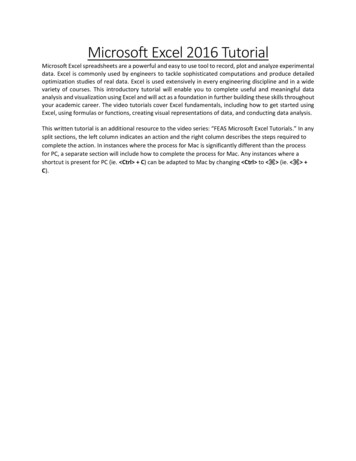
12Avoid common errors with formulasThe following table summarizes some of the most common errors that you can make when entering aformula and how to correct those errors:MAKE SURE THATYOU Match all open and closeparenthesesUse a colon to indicate arangeEnter all requiredargumentsNest no more than 64functionsEnclose other sheetnames in single quotationmarksEnter numbers withoutformattingMORE INFORMATIONMake sure that all parentheses are part of a matching pair. When you create aformula, Excel displays parentheses in color as they are entered.When you refer to a range of cells, use a colon (:) to separate the reference tothe first cell in the range and the reference to the last cell in the range. Forexample, A1:A5.Some functions have required arguments. Also, make sure that you have notentered too many arguments.You can enter, or nest, no more than 64 levels of functions within a function.If the formula refers to values or cells on other worksheets or workbooks, andthe name of the other workbook or worksheet contains a non-alphabeticalcharacter, you must enclose its name within single quotation marks ( ' ).Do not format numbers as you enter them in formulas. For example, even ifthe value that you want to enter is 1,000, enter 1000 in the formula.Charts in ExcelMicrosoft Excel no longer provides the chart wizard. Instead, you cancreate a basic chart by clicking the chart type that you want on theInsert tab in the Charts group. Charts are used to display series ofnumeric data in a graphical format to make it easier to understandlarge quantities of data and the relationship between different seriesof data.To create a chart in Excel, you start by entering the numeric data forthe chart on a worksheet. Then you can plot that data into a chart byselecting the chart type that you want to use on the Insert tab, in theCharts group.Worksheet dataChart created from worksheet dataGetting to know the elements of a chartA chart has many elements. Some of these elementsare displayed by default, others can be added asneeded. You can change the display of the chartelements by moving them to other locations in thechart, resizing them, or by changing the format. Youcan also remove chart elements that you do not wantto display.1The chart area is the entire chart and all itselements2The plot area is the area of the chart bounded bythe axes.Created By: Amy BeaucheminSource: office.microsoft.com1/13/11
13345The data points are individual values plotted in a chart represented by bars, columns, lines, or pies.67A chart and axis title are descriptive text that for the axis or chart.The horizontal (category) and vertical (value) axis along which the data is plotted in the chart.The legend identifies the patterns or colors that are assigned to the data series or categories in thechart.A data label provides additional information about a data marker that you can use to identify thedetails of a data point in a data series.Create a Chart1. On the worksheet, arrange the data that you want to plot in a chart. The data can be arranged inrows or columns — Excel automatically determines the best way to plot the data in the chart.2. Select the cells that contain the data that you want to use for the chart.NOTE: If the cells that you want to plot in a chart are not in a continuous range, you can selectnonadjacent cells or ranges as long as the selection forms arectangle. You can also hide the rows or columns that youdo not want to plot in the chart.3. Go to the Insert tab, in the Charts4. Click the chart type, and then click a chart subtype from the drop menu that will appear.5. Click anywhere in the embedded chart to activate it. When you click on the chart, Chart Tools willbe displayed which includes the Design, Layout, and Format tabs.6. The chart will automatically be embedded in the worksheet. A chart name will automatically beassigned.Move Chart to New Sheet1. On the Design tab, in the Location group, click Move Chart.2. Under Choose where you want the chart to be placed, click on the New sheet bubble3. Type a chart name in the New sheet box.Change Chart Name1. Click the chart.2. On the Layout tab, in the Properties group, click the Chart Name text box.3. Type a new chart name.4. Press ENTER.Change Chart Layout1. Click anywhere in the chart.2. Go to the Chart Tools, the Design group3. In the Chart Layouts, click the chart layout that you want to use. To see all available layouts, clickMoreCreated By: Amy Beauchemin.Source: office.microsoft.com1/13/11
14Change Chart Style1. Click anywhere in the chart.2. On the Design tab, in the Chart Styles group, click the chart style that you want to use. To see allpredefined chart styles, click More.Chart or Axis TitlesTo make a chart easier to understand, you can add titles, such as chart and axis titles.To add a chart title:1. Click anywhere in the chart.2. On the Layout tab, in the Labels group, click Chart Title.3. Click Centered Overlay Title or Above Chart.4. In the Chart Title text box that appears in the chart, type the text that you want.5. To remove a chart title, click Chart Title, and then click None.NOTE: You can also use the formatting buttons on the ribbon (Home tab, Font group). To format thewhole title, you can right-click it, click Format Chart Title, and thenselect the formatting options that you want.To add axis titles:1. Click anywhere in the chart.2. On the Layout tab, in the Labels group, click Axis Titles.3. Do one or more of the following:a. To add a title to a primary horizontal (category) axis, click Primary Horizontal Axis Title, andthen click the option that you want.b. To add a title to primary vertical (value) axis, click Primary Vertical Axis Title, and then click theoption that you want.4. In the Axis Title text box that appears in the chart, type the text that you want.5. To remove an axis title, click Axis Title, click the type of axis title to remove, and then click None.Data Labels1. On a chart, do one of the following:a. Click on the chart area to add a data label to all data points of alldata seriesb. Click in the data series to add a data label to all data points of adata seriesc. Click on a specific data point to add a data label to a single datapoint in a data series2. On the Layout tab, in the Labels group, click Data Labels, and thenclick the display option that you want.3. Text boxes will appear in the area of your chart based on your selection.4. Click on the text box to modify the text.5. To remove data labels, click Data Labels, and then click None.NOTE: Depending on the chart type that you used, different data labeloptions will be available.Created By: Amy BeaucheminSource: office.microsoft.com1/13/11
15LegendWhen you create a chart, the legend appears, but you can hide the legend or change its location afteryou create the chart.1. Click the chart in which you want to show or hide a legend.2. On the Layout tab, in the Labels group, click Legend.3. Do one of the following:a. To hide the legend, click None.b. To display a legend, click the display option that you want.c. For additional options, click More Legend Options, and then selectthe display option that you want.NOTE: To quickly remove a legend or a legend entry from a chart, you canselect it, and then press DELETE. You can also right-click the legend or alegend entry, and then click Delete.Move or Resize ChartYou can move a chart to any location on a worksheet or to a new or existingworksheet. You can also change the size of the chart for a better fit.To move a chart, drag it to the location that you want.To resize a chart, click on one of the edges and drag towards the center.Advanced Spreadsheet ModificationOnce you have created a basic spreadsheet there are numerous things you can do to make working withyou data easier. Some of these elements are hiding, freezing and splitting rows. You can also sort andfilter data, these features are quite helpful when working with a large amount of data.Hide or Display Rows and ColumnsYou can hide a row or column by using the Hide command or when you change its row height or columnwidth to 0 (zero). You can display either again by using the Unhide command. You can either unhidespecific rows and columns, or you can unhide all hidden rows and columns at the same time. The firstrow or column of the worksheet is tricky to unhide, but it can be done.Hide Rows or Columns1. Select the rows or columns that you want to hide.2. On the Home tab, in the Cells group, click Format.3. Under Visibility, point to Hide & Unhide, and then click HideRows or Hide Columns.NOTE: You can also right-click a row or column (or a selection ofmultiple rows or columns), and then click Hide.Unhide Rows or Columns1. Select the rows, columns or entire sheet to unhide.2. On the Home tab, in the Cells group, click Format.3. Under Visibility, point to Hide & Unhide, and then click UnhideRows or Unhide Columns.TIP You can also right-click the selection of visible rows andcolumns surrounding the hidden rows and columns, and then c
4. Click on Microsoft Excel 2010 Create a New Workbook 1. Click the File tab and then click New. 2. Under Available Templates, double click Blank Workbook or Click Create. Find and Apply Template Excel 2010 allows you to apply built-in templates and to search from a variety of templates on Office.com. To find a template in Excel 2010, do the .