WIXLIB

Microsoft Excel 2016 Tutorial In order to autofill cells:5Type in the first few entries into the column. Then,select all the column entries thus far by clickingthe middle of the topmost cell and dragging untilall the column entries are highlighted andsurrounded by the green border. Release the click,then move your cursor to the bottom right of yourselected cells where there is a small green square,changing the cursor to a black plus sign. Click anddrag down to populate as many lower cells as youintend.This method also works with days of the week, months and written patterns (such as Week 1, Week 2,Week 3 etc.).2.1.10 Sorting dataIt is often necessary to sort data in a spreadsheet according to one of the columns, for example fromsmallest to largest or vice versa.To sort data according to a specific scheme:Select all data columns and navigate to Sort in theSort and Filter group of the Data tab. Columnheadings can be included in the block as long asthe My data has headers box is ticked whenperforming the sort. Click the Sort button to bringup the Sort window. Next, use the drop downmenus to specify the criterion by which the data isto be sorted and in which order to you would likeit to be rearranged. The Options button can beused if you wish the sort to be case sensitive or tohave a special sort order such as days of the weekor months of the year. Once you’re satisfied withthe sort criteria, click OK.2.1.11 Transposing dataIt may be necessary to copy and paste a column of data into a row (or row to column) depending on thearrangement of your spreadsheet. A common instance of this transposition is the need to placeexperimentally obtained data from a data acquisition device into a worksheet that was set up prior toperforming the experiment.To transpose data:Copy the data then right-click on the first cell inwhich you wish the transposed data to be located.In the resultant Quick Menu, select Transposeunder the Paste Options.2.2 Using formulas and functionsNext we’re going to discuss formulas and functions. Formulas and functions in Excel are essential for theanalysis of data sets, and a firm grasp of this functionality will be invaluable in upper year laboratorycourses for any discipline.

Microsoft Excel 2016 Tutorial 62.2.1 Custom formulasWe’ll start with custom formulas. Excel can be used to perform custom mathematical operations on datasets.To perform a custom mathematical operation:Select the cell and begin by typing “ ”. Useparentheses, operations ( , -, *, /, ) and click oncells you wish to reference in the formula, andevaluate the cell by pressing Enter .For example, if you wish for the contents of cell B3 to be twice the value of cell A3, cell B3 would containthe following formula: “ A3*2”. When you press Enter , cell B3 will evaluate and the formula willdisappear.To edit a formula:Select the cell and press F2 or click in the formulabar just above the column headers.2.2.2 Built-in FunctionsExcel also has built in functions for a number of mathematical operations; a few illustrative functions areincluded below in Table 1. Functions are usually common mathematical actions that are challenging towrite formulas for (such as finding the average or mean of a dataset or calculating the sine of an angle).Entering a function is similar to a formula:Type ‘ ’ then follow with the desired function. Enter will evaluate the cell.The Excel help menu and online forums give detailed information on all available built in functions. Usingfunctions can greatly speed up completing calculations and prevent human error in entering formulas.Table 1: A few examples of built-in functions in ExcelNameSyntaxActionSumAverageSineSUM(element1, element2 )AVERAGE(element1, element2 )SIN(angle)Sums all the elements in parenthesisFinds the average of the input elementsFinds the sine of a given angle2.2.3 Copying formulas/functionsIt is often useful to apply the same formula to a column of data. This can be achieved using two methods:the click and drag trick or copy and paste.Select the cell containing the original formula,then move the cursor to the bottom right cornerof the cell where the small green square is located,changing the cursor to a black plus sign ( ). Clickand drag the cursor down to the last row in whichyou want the formula, or double-click to have theformula populate automatically to the lowest rowwith data.

Microsoft Excel 2016 Tutorial To Copy and paste formulas and functions:7Select the cell to copy and press Ctrl and C andthen paste it in the cells intended for evaluationusing Ctrl and V.2.2.4 Absolute and relative referencingWhen copying a formula to multiple rows, Excel will keep shifting the cells used in the formula down byone row. This is called relative referencing and is Excel’s default for copying formulas and functions. If youwish to always evaluate a formula or function with reference to the value in one specific cell, this is calledabsolute referencing.To use absolute referencing in a formula:Take the cell reference that you intend to makeabsolute (for example B4) and add ‘ ’ symbolsbefore the value (row and/or column) that youwant to fix. Thus B4 becomes B 4 if you want tofix both the row and column, while B4 becomesB 4 if you only want to fix the row (4).3. Data visualizationIn this section we are discussing data visualization. This section covers how to create a scatter plot andhow to properly format graphs. To describe these concepts, data from an example lab is used. Theconcepts and data discussed in this section are entirely for illustratory purposes so don’t worry aboutunderstanding the physics, just focus on the Excel skills.In this example lab, you are asked to compare the Elasticity of a ping-pong ball and a rubber ball. Elasticityis defined as the ratio of bounce height, ℎ𝑏 , to initial drop height, ℎ𝑖 . The initial drop height and bounceheights along with the associated measured error of the rubber ball and the ping-pong ball can be seen inTable 2.Table 2: Experimental data for the bounce heights of the rubber ball and ping pong ball.Trial#123456789Rubber BallhrihriError 700.557800.566900.5721000.581hrb[cm]222222222Ping Pong BallError hpihpiError 700.547800.551900.5601000.567hpb[cm]222222222Error

Microsoft Excel 2016 Tutorial .57580868222In this scenario, it is expected that the initial and bounce heights relate according to the followingequation:ℎ𝑏 𝐸ℎ𝑖where ℎ𝑏 is the bounce height (in m), E is the elasticity of the ball (dimensionless), and ℎ𝑖 is the initial dropheight (in m). It should be noted that this relationship resembles the equation of a straight line intersectingthe origin. We will determine whether our collected data fits this linear model using graphs forvisualization.3.1 Inserting a scatter plotThe Scatter Plot will be used for many future engineering applications, and plots each data pointseparately on the chart area. Do not confuse it with the Line Chart, which is similar but uses lines toconnect data points. It should be noted that in the example lab the initial height, hi, is the independentvariable and should be placed on the horizontal axis, whereas the bounce height, hb, is the dependentvariable and thus should be placed on the vertical axis. The concepts of dependent and independentvariables will be explored further in other courses.To insert a scatter plot:Go to the Charts group in the Insert tab and selectScatter.Note that an inserted plot will be blank until you add one or more data series to the plot area.3.2 Selecting data seriesThe next step is to add a data series to the blank To do this, right-click on the blank plot and click onplot:Select Data in the Quick Menu. In the SelectData Source window, click on Add. Give adescriptive name in the Series Name dialogue box(in the example lab we’ll plot the rubber ball datafirst and thus will type Rubber Ball into the box).In the Series X values dialogue box, click theCollapse button beside the box. Now, select all thenumbers (the column under the column header)representing the hri values for the rubber ball, thenpress Enter to return to the Edit Series window.In the same manner, select all the hrb values for therubber ball for the Series Y values. Click OK toreturn to the Select Data Source window then clickOK again.If the resultant plot is sitting on top of your data table, simply click and drag the plot window away fromthe data to another location in your spreadsheet.

Microsoft Excel 2016 Tutorial 9It is now time to add the second set of data points to the same graph. Use the same procedure as that ofthe rubber ball to add the series for the ping pong ball. The resultant graph should possess two sets ofdata; however, it needs to be formatted to look professional.3.3 Chart formattingAn essential aspect of data visualization is proper formatting. An improperly formatted chart will likelynot describe data in an adequate manner.3.3.1 Title, legend, labelsAlways add a title, axis labels, and a legend to your scatter plot. It should be noted that in professionalreports, titles are NOT included on graphs; however, it is useful to include titles in your Excel worksheetto improve readability. To delete the title when you copy the Excel plot into Microsoft word during yourreport write up, simply select the title and press Delete .To add a title, legend and labels:Left-click anywhere on the chart and note that agreen plus sign appears at the top left corner. Clickon the green plus sign and check off the Axis Titles,Chart Title and Legend boxes. The small arrow tothe right of the boxes allows for specifications ofeach addition. This addition of elements can alsobe accomplished by selecting the Add ChartElement in the Chart Layouts Group of the ChartTools tab that appears at the top of the windowwhen a graph is selected. Type in your own chartand axis titles by clicking on the titles in the graph.Make sure to include units in the axis titles.3.3.2 Tick marksIt’s useful to tidy up the axis by displaying major and minor tick marks. This will clarify data ranges andimprove the readability of the plot.To alter tick marks:Right-click on the vertical axis line, then selectFormat Axis. A toolbar will appear on the right sideof the window. Under the Tick Marks section, usethe drop down menu to change Major type toInside. Repeat this procedure for the horizontalaxis tick marks.3.3.3 Axis rangesData should always be spread evenly across a plot area, as opposed to being bunched in one half of achart. Bunching can be fixed by altering the axis ranges.To modify the horizontal and vertical axis ranges Right-click on the vertical axis, and then selectand specify the types of numbers on the graph:Format Axis. In the Axis Options section, changethe Bounds. This sometimes takes some playingaround to get a nice spread of data. In the samplelab, having a Minimum of 0 and a Maximum of120 produces an aesthetically pleasing plot. Note

Microsoft Excel 2016 Tutorial 10that you can always reset the axes to the initialauto-generated range by clicking the Reset buttonnext to Minimum and Maximum. Under theNumber section, you can specify what Type ofnumber the axis represents, and change thedisplayed number of decimals on the major tickmarks. Repeat this procedure for the horizontalaxis.3.3.4 Gridlines and border stylesAnother formatting option is to alter gridlines and border styles. There is no standard formatting for this,so feel free to play around. However, always make sure that formatting makes your chart easier to readand understand.To format the gridlines and the border styles:Right-click on the horizontal gridlines (inside thegraph axes) and then select Format Gridlines.Under Dash Type, select the Dash option. You mayhave to add vertical gridlines by right-clicking onthe horizontal axis, then selecting Add MajorGridlines before formatting them to the dashedline. Then, right-click on the white space withinthe plot area and select Format Plot Area from theQuick Menu. Under the Border section, selectSolid line.3.3.5 Error barsThe last, and extremely important step in presenting data is the addition of error bars on each of thepoints in accordance with the specified uncertainty. In the example lab, error for each point is specifiedin Table 2. Error bars for each series will be added separately.The process for adding error bars to data is different in Excel for Mac, therefore a section is includedhighlighting difference in this process when using Excel for Mac.The first step is to open the Error Bar Options To do this, click on any of the rubber ball datatoolbar:points to highlight all the points in the series.Under the Chart Tools - Design tab, select the AddChart Element button in the Chart Layouts groupin the top left corner. Under Error Bars, selectMore Error Bars Options to bring up the toolbaron the right side of the window. In bold green,Excel will specify whether you are formatting theVertical Error Bar or the Horizontal Error Bar. Toswitch between the two, click the bolded Error BarOptions drop down at the top of the toolbar andselect between Series “Rubber Ball” X Error Bars orSeries “Rubber Ball” Y Error Bars.

Microsoft Excel 2016 Tutorial 11Next , you need to select the correct type of error: If the error amount is the same for all data points,the easiest method is to type in the uncertainty inthe Fixed Value box under Error Amount. ThePercentage box may also be used if the error isalways some fixed percentage of the value. Inmost cases, the error amounts will differ for eachdata point and may even differ between thepositive and negative errors. Thus, the formattingof error bars requires use of the Custom button.To add custom error bars:Select the Custom button and then click theSpecify Value button. This action will bring updialogue boxes for the positive and negative errorsthat work in the same manner as selecting data.The order in which the error data is selectedcorresponds to the points on which the error barswill be placed in your graph (first selected cellcorresponds to error on the first data point in theseries, second cell corresponds to error on second,etc.). Click the Collapse button beside the positiveerror box and then select all the errors for thebounce heights of the rubber ball, then press Enter . In this case, the error for the bounceheight is 2cm, and thus the positive and negativeerrors for the bounce height are the same. As aresult, the negative errors can be specified by thesame cells as the positive errors. Click OK afterspecifying both errors, but do NOT close thetoolbar on the right side of the window. Now clickthe bold Error Bar Options drop down as before tobring up the Series “Rubber Ball” X Error Bars andrepeat the same procedure.The last step is to format the data markers to make To reduce the size of the data point markers, thuserror bars easier to read:making the error bars more visible, right-click onany of the markers then select Format DataSeries to bring up the right side toolbar.Underneath the bolded Series Options title, clickthe Fill & Line (paint can) button, then clickMarker. Under Marker Options, change themarker type to Built-in and specify an appropriatemarker size (4 is usually a good size). Repeat thesame error bars procedure for both seriesmarkers. It should be noted that you can also alterthe format of the error bars in a similar manner byright-clicking on an error bar.

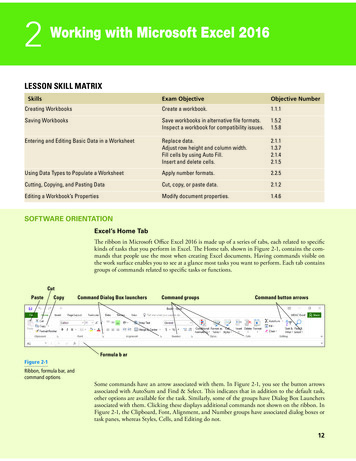
Microsoft Excel 2016 Tutorial 12A properly formatted graph of the ball data, created by following the above steps, is shown below in Figure1.3.3.5.1 Error Bars for MacThe process for adding error bars in Excel for Mac is very similar, with the sole exception being openingthe Error Bar Options toolbar.To open the Error Bar Options toolbar in Excel for Click on any of the rubber ball data points toMac:highlight all the points in the series. Under theChart Layout tab, select the Error Bars button inthe Analysis. Under the drop down menu, selectError Bars Options to bring up the window.Select the Error Bars tab.After this step, follow the same process described above to select the appropriate type of error and addthe bars for both the x and y axis error. Regardless of your version of Excel, a properly formatted graphshould look like the one included below in Figure 1.Elasticity of Two Ball Types120Bounce Height [cm]1008060Rubber BallPing Pong Ball40200020406080100120140Initial Height [cm]Figure 1: The final plot of the ball lab, showing both rubber and ping pong ball data3.4 Extracting tables and graphsTo display plots and tables in your report, you need to move them from Excel in to Microsoft Word. Whenyou bring your tables and graphs from Excel to Word for the creation of your reports, the default is for alink between the Word table or graph and the Excel table or graph. This default means that when thetable or graph is updated in Excel, it will also be updated in Word. Because of this link there is the potentialfor Word to run slowly, particularly for large documents with many linked figures and tables. To avoid thisdelay, there is the ability to copy a table or graph into Word as a picture.

Microsoft Excel 2016 Tutorial 13To copy a table or graph:Instead of simply using Ctrl and V to paste agraph into your Word document, right-click whereyou wish to paste the table or graph, then selectPaste as Picture from the Paste Options. You mayneed to format the picture to fit within themargins of your page.4. Data analysis4.1 Linear regressionMany engineering labs and projects involve fitting a mathematical model or equation to experimentaldata. This analysis may be done to determine the effect of one variable on another, such as therelationship between drop and bounce heights explored in the example lab. When dealing with linearrelationships, the best method to “draw” the perfect line is to use linear regression. The theory behin

Microsoft Excel 2016 Tutorial Microsoft Excel spreadsheets are a powerful and easy to use tool to record, plot and analyze experimental data. Excel is commonly used by engineers to tackle sophisticated computations and produce detailed optimization studies of real data. Excel is used