WIXLIB

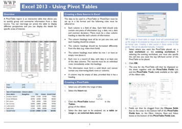
Excel 2013 - Using Pivot TablesOverviewCreating a Data Source in ExcelA PivotTable report is an interactive table that allows youto quickly group and summarise information from a datasource. You can rearrange (or pivot) the table to displaydifferent perspectives and you can display the details forspecific areas of interest.The data to be used in a PivotTable or PivotChart must beset up in a list format and the following rules must beadhered to: Each column is a field of data. Each field should onlycontain one piece of information (e.g. a date, not a dateand contract duration.) There must be a clear columnheading to describe each column of information. The column headings must all be on just one row, andeach heading should be unique. The column headings should be formatted differentlyfrom the data (e.g. make them bold) The column headings must either be row 1 or have anempty row above it. Each row is a record of data, with data in at least oneof the data columns. The records must be on individualrows, immediately under the headings.From this . .to this The information must form a solid block and cannotcontain any intervening blank rows or columns. A column may be empty of data, provided that it has aheading.TIP If using an Excel table or range, Excel will automatically pickup the range to be analysed as long as your data is in a recognisedlist format (see, Creating a data source in Excel earlier in thisguide). This can be adjusted manually, if required.5. Select where you want the PivotTable placed, viz. anew worksheet or, the existing worksheet. Ifselecting the existing worksheet, you must also specifythe cell into you want the top left-hand corner of thePivotTable to be placed.6.Click OK.7.The area for the PivotTable will then be displayed onthe sheet, together with the PivotTable Fields Listand the PivotTable Tools made available at the rightof the ribbon tabs.8.Fields can then be dragged from the Choose fieldsbox to the areas in the bottom half of the PivotTableFields box, to the Filters, Columns, Rows and Valuesboxes at the bottom of the PivotTable Fields List.Creating a PivotTable1.Select any cell within the range of data.2.Select the Insert tab.3.Click the PivotTable buttonTablesgroup of the ribbon.4.Select the data type to be analysed, viz. a table orrange or, an external data source.1in the

Excel 2013 - Using Pivot TablesUse the Rows and Columns areas to summarize the datainto groups. You can use both areas, if desired.Use the Values area to create summary calculations at theintersection of each row and/or column. By default, thevalue area will sum numeric data or count text data. Thesecan, if desired, be changed later.Use the Filters area to filter data by selecting a value froma drop-down list.As you add fields to these boxes, Excel will construct thePivot table by grouping data in the Row Labels field(s) intothe Row area, the Column Labels field(s) in the Columnarea. Fields placed in the Value box will be added to theData area and fields added to the Filters box will appear inthe area above the pivot table.In the example below, Full Name has been placed in theRows box, Type in the Columns box, Amount in the Valuebox and Region in the Filters box.Will subdivide Regions into each Salesperson.7.Add to ValueAdd to FiltersUsing multiple fields1.Additional fields can be added to the Filters,Columns, Rows and Value areas.2.Click onto the PivotTable that you want to add fieldsto. This will activate the PivotTable Field List and thePivotTable Tools.3.Drag and drop your chosen fields from the Choosefields to add to report: list into the appropratebox(es) at the bottom of the PivotTable Fields List.4.Look out for the blue/green line as as you click anddrag the field over the boxes. The position of this linewill affect how the data is displayed on the PivotTable.For example:Moving a field1.If you add more than one data field into an area, youcan arrange the fields in the order that you want.2.At the bottom of the PivotTable Fields List, clickthe drop-down arrow at the right of the field that youwant to move.Select the appropriate Move (Up;Beginning; to End etc.) command.3.Down;toOR4.5.Will subdivide each Salesperson group into Types.Click and drag the field header from one box toanother. For example, you could drag a field from theColumns box to the Rows box, or drag one fieldname above another if the area contains more than onefield.Removing a fieldTIP: Alternatively, items can be ticked in the Choose fields to addto report: list in the PivotTable Field list directly onto thePivotTable into the Drop Page Fields Here, Drop Column FieldsHere, Drop Row Fields Here and Drop Data Items Here areas.If you decide to drag fields directly into the PivotTableareas, look out for the following symbols on the mousepointer:6.Whereas:1.Click and drag the field header out of the PivotTablefields box. The following symbol next to the mousepointer will indicate that it is in the right position forthe field to be removed .2.OR:3.At the bottom of the PivotTable Field List, click thedrop-down arrow at the right of the field that you wantto remove.4.Select Remove Field.Add to RowAdd to Column2

Excel 2013 - Using Pivot TablesOrganising PivotTable DataFilteringWhen a PivotTable has beencreated, items can be hiddenfrom the Row or Columnareas by clicking the dropdown arrow at the end of theheading and unchecking itemsto be hidden or shown.Remember to click OK.The Page area may be used in asimilar way but selecting an entryfrom the list will filter out all datanot meeting this criteria when youclick OK.Viewing underlying recordsPivot table OptionsAdditional options for fine-tuning and setting preferencesfor how your PivotTable works can be found by:1.Clicking the Analyze tab of the PivotTable Tools onthe Ribbon.2.Clicking the Options button in the PivotTable group.3.Two of the most useful of these are:4.Totals & Filters tab - Show grand totals for rows (orcolumn). This allow you to decide whether each rowor column of data has a total at the right (for rows) orat the bottom (for columns).5.Double clicking a value in the Data area, will give you abreakdown of the figures used to make up the value on aseparate sheet.SortingBy default, data will be shown in ascending order fornumbers or A-Z for text. If you amend or add new datayou may wish to re-sort data or adjust the sort order.1.Click the drop-down arrow at the right of the fieldheader that you want to sort on.2.Click Sort A to Z, Sort Z to A or More SortOptions Data tab - Refresh data when opening the file. This willautomatically refresh its view of the data when youopen the workbook. Please note that this will notautomatically extend the data range to new data (seeAdding data to your PivotTable, later in this guide).Modifying the Value Field‘s CalculationsBy default, in the Value area, numeric values are summedand text values are counted. The get the PivotTable tocarry out a different calculation on the data:1.At the bottom of the PivotTable Fields List, clickthe down-arrow at the right of the value field button.2.Select Value Field Setting .3.From the Summarize values by: list select the typeof calculation required4.Click OK.5.OR6.Right-click one of the values and select SummerizeData ByMultiple Data fieldsYou can add a field more than once to the Data area andset the first instance to sum and the second to count so asto show the total value and the number of instances1.In the PivotTable Fields List, add the field for thesecond calculation to the Value area.2.Click the down-arrow at the right of the value fieldbutton.3.Select Value Field Setting .4.From the Summarize values by: list select the typeof calculation required5.Click OK.NB: The field summary heading will change e.g. from Sum of ,field name to Count of field name .3

Excel 2013 - Using Pivot TablesAdding Data to your PivotTableFormatting a Pivot TableWhen you amend any of the data within the range of datacurrently being used to generate the PivotTable or Chartyou must refresh the PivotTable. If you add extra data tothe range you will need to adjust the PivotTable’s datarange.A PivotTable can be formatted like any other spreadsheet. Ifyou format cells, then check that the Pivot Table optionPreserve cell formatting on update is turned on.Refreshing data1.Select a cell on the PivotTableSelect any cell on the PivotTable.2.2.Click the Options tab in the PivotTable Toolssection of the Ribbon.Select the Design tab in the PivotTable Toolssection of the ribbon.3.Click a button in the PivotTable Styles group of theribbon.3.Click the Refresh button in the Data group.Adding dataWhen you created the Pivot Table you specified a range ofdata to be plotted. If you add new data at the end of yourlist, you will need to adjust the PivotTable’s data range.Merely using the Refresh button does not do this!1.Select any cell on the PivotTable2.Click the Options tab in the PivotTable Toolssection of the Ribbon.3.Click Change Data Source in the Data group.Tip: Moving the mouse pointer over the styles will preview thestyle on the PivotTable. The style, however, is only appliedwhen the button is clicked.4. Fine-tune a style by checking and/or unchecking the tickboxes in the PivotTable Style Options group of theribbon.Tip: To reset the PivotTable style to the default, select the “None”style in the top left of the PivotTable styles button.Pivot ChartsA Pivot Chart is an interactive graphical representation ofthe data in a Pivot able.You can rearrange the layout, select a different type ofchart, and add or remove data.4.5.Click the PivotChart button in the Charts group4.Select the data type to be analysed, viz. a table orrange or, an external data source.AutoFormatting a PivotTable1.NB: The button has a drop-down arrow from which you canselect Refresh All. This will refresh ALL PivotTables in theworkbook which are based on the same source data as theselected one.4. The PivotTable(s) will be re-drawn to show theamended data3.Creating a PivotChart from scratchType or re-select the data range upon which to basethe amended Pivot Table.1.Select any cell within the range of data.Click OK.2.Select the Insert tab.4TIP If using an Excel table or range, Excel will automaticallypick up the range to be analysed as long as your data is in arecognised list format (see, Creating a data source in Excelearlier in this guide). This can be adjusted manually, ifrequired.1. Select where you want the PivotChart placed, viz. anew worksheet or, the existing worksheet. Ifselecting the existing worksheet, you must also specifythe cell into you want the top left-hand corner of thePivotChart to be placed.2.Click OK.3.The area for the PivotChart will then be displayed onthe sheet, together with the PivotTable Field List, aPivotChart Filter Pane and a PivotChart Toolssection at the right of the ribbon tabs.NB: As well as the new PivotChart a new PivotTable will havebeen created, the two are permanently linked1. Fields can then be dragged from the Choose fields toadd to report: list in the PivotTable Field list, tothe Filters, Legend (Series) , Axis(Categories), and Valuesboxes at the bottom of the PivotTable Field List.Use the Axis Fields area to specify what the PivotChartgroups and displays along the horizontal (x) axis.