Transcription
Revision 1 (06-2015)Microsoft Excel 3Advanced-Level Features of Excel 2013Pivot TablesSee the Pivot Tables tab in the Excel 3 Practice.xls spreadsheet located on the Workshop documentsfolderPivot tables in Excel are a versatile reporting tool that makes it easy to extract information from large tables ofdata without the use of formulas. Pivot tables are extremely user-friendly in that by moving (or pivoting) fieldsof data from one location to another using drag-and-drop we can look at the same data in a number of differentways.1. Add the data you wish to create a pivot table for. Sample data (in cells A2 to D12) has already beenentered for you in the Pivot Tables tab in the Excel 3 Practice.xls spreadsheet. Note that your datahas multiple columns so you can view the data multiple ways. At least three columns of data are neededto create a pivot table. Do not leave blank rows or columns when entering the data. Also, do not leave ablank row between the column headings and the first row of data.2. Left-click-and-drag the sample data from cells A2 to D12 to highlight just the column headers and thedata. Do not highlight the cell A1 containing ‘Cookie Sales by Region’.3. Click on the Insert tab of the Ribbon at the top of Excel.4. Click on the down arrow at the bottom of the Pivot Table button to open the drop-down list.5. Click on Pivot Table in the list to open the Create Pivot Table dialog box.6. Click on Existing Worksheet for the location of the pivot table.7. Click on the Location line in the dialog box.This work was created by PPL.This work is licensed under a Creative Commons Attribution-Noncommercial-Share Alike 3.0 License. You are free to copy, distribute, transmit, and adaptthis work provided that this use is of a non-commercial nature, that any subsequent adaptations of the work are placed under a similar license, and thatappropriate attribution is provided where possible.Page 1 of 13
8. Click on cell A16 in the worksheet to enter that cell reference into the location line.9. Click the OK button.10. A blank pivot table object (like the one below) should appear on the worksheet with the upper-leftcorner of the pivot table in cell A16.11. The Pivot Table Field List should open on the right-hand side of the Excel window. At the top of thePivot Table Field List are the field names (column headers) from our data table. The data areas at thebottom of the panel are linked to the pivot table.12. Now you will configure (add data to) the pivot table by dragging and dropping the field names to thedata areas within the Pivot Table Field List as follows: Drag the Total Sales field to the Report Filter area Drag the Region field to the Column Labels area Drag the Sales Rep field to the Row Labels area Drag the # Orders field to the Values area13. Click on cell A17 and in the Formula Bar, rename it from Row Labels to Sales Rep.14. Click on cell B16 and in the Formula Bar, rename it from Column Labels to Region.15. After completing the above step, your pivot table should look like the one located in cells H14 to M28(and shown below) and the Pivot Table Field List should look like the picture below.This work was created by PPL.This work is licensed under a Creative Commons Attribution-Noncommercial-Share Alike 3.0 License. You are free to copy, distribute, transmit, and adaptthis work provided that this use is of a non-commercial nature, that any subsequent adaptations of the work are placed under a similar license, and thatappropriate attribution is provided where possible.Page 2 of 11
16. Try using the drop-down filter buttons for Sales Rep and Region to hide selected data rows andcolumns.This work was created by PPL.This work is licensed under a Creative Commons Attribution-Noncommercial-Share Alike 3.0 License. You are free to copy, distribute, transmit, and adaptthis work provided that this use is of a non-commercial nature, that any subsequent adaptations of the work are placed under a similar license, and thatappropriate attribution is provided where possible.Page 3 of 11
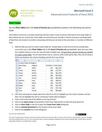
17. Try creating a new pivot table like the one located in cells H3 to S11 (shown below) by configuring thepivot table like the picture below. Note that you can either create a new pivot table or simply just dragand drop the field names in your old pivot table to the different data areas shown below.Drag the field names todifferent data areas toobtain different viewingresults from the PivotTableThis work was created by PPL.This work is licensed under a Creative Commons Attribution-Noncommercial-Share Alike 3.0 License. You are free to copy, distribute, transmit, and adaptthis work provided that this use is of a non-commercial nature, that any subsequent adaptations of the work are placed under a similar license, and thatappropriate attribution is provided where possible.Page 4 of 11
Removing Duplicate Data RecordsSpreadsheet programs such as Excel are often used as databases for things like parts inventories, sales records,and mailing lists. Databases are normally organized into rows of data called records. In a record, the data in eachcell or field in the row is related - such as a company's name, address and phone number. A common problemthat occurs as a database grows in size is that of duplicate records.This duplication can occur if: entire records are entered into the database more than once resulting in two or more identical records multiple records have one or more fields - such as a name field or address - containing the same data.Either way, duplicate records can cause a whole host of problems so it's a good idea to scan for and removeduplicate records on a regular basis. To help you accomplish this task Excel has a built in data tool called, notsurprisingly, Remove Duplicates.1. Add the data you wish to use, along with duplicate records. Sample data (in cells A1 to C15) has alreadybeen entered for you in the Duplicate Data tab in the Excel 3 Practice.xls spreadsheet (image ofdata is shown below):2. Click on any cell containing data in the sample database in cells A1 to C15.3. Click the Data tab on the Ribbon.4. Click on the Remove Duplicates icon to highlight all data in the database and to open the RemoveDuplicates dialog box.This work was created by PPL.This work is licensed under a Creative Commons Attribution-Noncommercial-Share Alike 3.0 License. You are free to copy, distribute, transmit, and adaptthis work provided that this use is of a non-commercial nature, that any subsequent adaptations of the work are placed under a similar license, and thatappropriate attribution is provided where possible.Page 5 of 11
5. Leave a checkmark only in the Student ID column. Remove the checkmarks from the Student Name andClassification columns. Leave the checkmark in the My data has headers checkbox. Click on the OKbutton.6. After removing the duplicate data, your data should look like the image below. Note that removingduplicate data does not automatically sort the remaining data records for you.SparklinesWhat is a sparkline?A sparkline is a small chart that is aligned with rows of some tabular data and usually shows trend information.Sparklines (often called as micro-charts) add rich visualization capability to tabular data without taking too muchspace. They have also been referred to as intense, simple, word-sized graphicsHere is an example of sparklines in a project team status report with sparklines displayed in cells B2 through B7.1. Click on the Insert tab.2. Select the data from which you want to make a sparkline. Left-click and drag on cells C2 through K43. In the Sparklines group, click on the Line buttonThis work was created by PPL.This work is licensed under a Creative Commons Attribution-Noncommercial-Share Alike 3.0 License. You are free to copy, distribute, transmit, and adaptthis work provided that this use is of a non-commercial nature, that any subsequent adaptations of the work are placed under a similar license, and thatappropriate attribution is provided where possible.Page 6 of 11
4. Specify a target cell(s) where you want the sparkline(s) to be placed. In the Create Sparklines dialog boxwith the cursor blinking in the Location Range textbox, left-click and drag on cells B2 through B4 andthen click the OK button5. Optional: Format the sparkline(s), if you so desire. With the new sparkline(s) still highlighted, click thedown-arrow next to the Sparkline Color (located in the Style Group) and choose a color. Click the downarrow next to the Marker Color (located in the Style Group) and choose colors for High Point (choosegreen), Low Point (choose red) and Markers (choose black).6. Click on the Insert tab then left-click and drag on cells C5 through K77. In the Sparklines group, click on the Column button then left-click and drag on cells B5 through B7 thenclick on the OK button8. Format the Sparkline Color and the Marker Color similar to the colors used in Step 5 above9. At a later date, if you wish to change colors or line types for the sparkline simply click on the sparklineand Excel will change to the Design tab to allow you to make your new choices.Excel Drop-Down ListExcel's data validation options include creating a drop down list that limits the data that can be entered into aspecific cell to a pre-set list of entries.The benefits for using a drop down list for data validation include: making data entry easierpreventing data entry errorsrestricting the number of locations for entering dataWhen a drop-down list is added to a cell, an arrow is displayed next to it. Clicking on the arrow will open the listand allow you to select one of the list items to enter into the cell. See the image below:This work was created by PPL.This work is licensed under a Creative Commons Attribution-Noncommercial-Share Alike 3.0 License. You are free to copy, distribute, transmit, and adaptthis work provided that this use is of a non-commercial nature, that any subsequent adaptations of the work are placed under a similar license, and thatappropriate attribution is provided where possible.Page 7 of 11
The items that are added to the list can be located on the same worksheet as the list, on a different worksheetin the same Excel workbook, or can be entered directly into the list. In this tutorial we will create a drop downlist using a list of entries located on the same worksheet as the drop-down list itself.1. The first step to creating a drop-down list in Excel is to enter the list data. In order to save time, the listdata has been pre-entered for you in cells A3 through A25 in the Drop-Down List tab in the Excel 3Practice.xls spreadsheet (image of data is shown below). Note that cell A3 is empty and willshow up as a blank line in the first position in the data list. Note that some people prefer to placethe list data in a separate spreadsheet or move it out of sight within the same spreadsheet where thedrop-down listbox is placed. For ease of use, we have placed the list data in close proximity to the dropdown listbox.2. Click on cell B1 to make it the active cell - this is where the drop down listbox will be located.This work was created by PPL.This work is licensed under a Creative Commons Attribution-Noncommercial-Share Alike 3.0 License. You are free to copy, distribute, transmit, and adaptthis work provided that this use is of a non-commercial nature, that any subsequent adaptations of the work are placed under a similar license, and thatappropriate attribution is provided where possible.Page 8 of 11
3. Click on the Data tab in the ribbon menu and select the Data Validation button4. In the Data Validation dialog box that popped up, choose List for the Allow: entry, un-check the box byIgnore blank and then click in the Source box (match the settings from the image above)5. Left-click-and-drag on cells A3 through A25 to select the range for the Source box. Note that if youprefer to enter data directly into the Source line of the dialog box, the list items must be separated by acomma such as: Animal Crackers, Biscuit, Butter Cookie, Chocolate Chip6. Click on the OK button to close the dialog box7. Now, when you left-click on the drop-down arrow for the listbox, you should see something like theimage below:Creating plots of multiple data series on one chart/graphLet’s say that you have monthly sales data for the entire year of 2013 for three salespeople and you would liketo show all three sales data series in different colors on the same chart/graph. Some random data has been preentered for you in cells A2 through D15 in the Multiple Series Chart tab in the Excel 3 Practice.xlsThis work was created by PPL.This work is licensed under a Creative Commons Attribution-Noncommercial-Share Alike 3.0 License. You are free to copy, distribute, transmit, and adaptthis work provided that this use is of a non-commercial nature, that any subsequent adaptations of the work are placed under a similar license, and thatappropriate attribution is provided where possible.Page 9 of 11
spreadsheet (image of data is shown above). Note that when you save the spreadsheet, new randomdata will automatically be generated for you.1. Click on the Insert tab in the ribbon menu and go to the Charts group and select the Insert Scatter (X, Y)or Bubble Chart button and choose Scatter with Straight Lines and Markers2. Right-click on the blank chart and choose Select Data then click on the Add button in the Select DataSource dialog box.3. Type in Dave for the Series name: field then click in the Series X values: field and left-click and drag oncells A4 through A154. Click in the Series Y values: field then highlight any data in that field and press the delete key. Left-clickand drag on cells B4 through B15 and click on the OK button5. Click on the Add button again in the Select Data Source dialog box and repeat Steps 3 and 4 using Jimfor the Series name and cells A4 through A15 for the Series X values and cells C4 through C15 for theSeries Y values and click on the OK button.6. Repeat Step 5 using Mary for the Series name and cells A4 through A15 for the Series X values and cellsD4 through D15 for the Series Y values and click on the OK button. Click on the OK button in the SelectData Source dialog box.7. Add a Chart Title for the horizontal axis by clicking on Add Chart Element in the upper-left corner of theDesign tab. Select Axis Title then Primary Horizontal and then type in Month and press the Enter key8. Add a Chart Title for the vertical axis by clicking on Add Chart Element in the upper-left corner of theDesign tab. Select Axis Title then Primary Vertical and then type in Sales and press the Enter key9. Click on the chart to select it then click on the sign button to the right of the chart.This work was created by PPL.This work is licensed under a Creative Commons Attribution-Noncommercial-Share Alike 3.0 License. You are free to copy, distribute, transmit, and adaptthis work provided that this use is of a non-commercial nature, that any subsequent adaptations of the work are placed under a similar license, and thatappropriate attribution is provided where possible.Page 10 of 11
10. In the Chart Elements dialog box, put checkmarks in the Chart Title and Legend checkboxes and thenclick in an empty cell.11. Double-click on Chart Title textbox and replace Title with 2013 Monthly SalesSample Monthly Budget and Spending PlanSee the Dec 2013 Spending Plan tab and the Dec 2013 Budget in the Excel 3 Practice.xls spreadsheet.During class we will add some more sample data to these spreadsheet to demonstrate the formula-basedconditional formatting and some what-if scenarios.Northstar ReviewSee the Northstar Review tab and go through the steps numbered 1 through 13. These questions arerepresentative of questions that will be on the northstar.This work was created by PPL.This work is licensed under a Creative Commons Attribution-Noncommercial-Share Alike 3.0 License. You are free to copy, distribute, transmit, and adaptthis work provided that this use is of a non-commercial nature, that any subsequent adaptations of the work are placed under a similar license, and thatappropriate attribution is provided where possible.Page 11 of 11
Advanced-Level Features of Excel 2013 Pivot Tables See the Pivot Tables tab in the Excel 3 Practice.xls spreadsheet located on the Workshop documents . In this tutorial we will create a drop down list using a list of entries located on the same worksheet as the drop-down list itself. 1. The first step to creating a drop-down list in Excel is .