WIXLIB

Two-Way Independent Samples ANOVA with JMP Obtain the file ANOVA2.jmp from my JMP data page. The data are those that appear in Table17-3 of Howell’s Fundamental statistics for the behavioral sciences (7th ed.) and in Table 13.2 ofHowell’s Statistical methods for psychology (7th ed.). Dr. Howell created these data so that thegroups (cells) would have the same means and standard deviations obtained by Eysenck. Youshould read the original research article: Eysenck. M. W. (1974). Age differences in incidentallearning. Developmental Psychology, 10, 936 – 941. The independent/grouping/classificationvariables are age of participant (young or old) and depth of cognitive processing (manipulated by theinstructions given to participants prior to presentation of a list of words). Thedependent/outcome/comparison variable is number of words correctly recalled later.First we need to get some basic descriptive statistics. From the data window, select Tables,Tabulate. In the dialog window, select Items and then drag Items to the “Drop zone for columns” anddrop it there. When prompted, select “Add analysis columns.”Next, select N, Mean, and Std Dev in the pane of statistics. They will be highlighted in blue.Drag this block of selected statistics on top of “Sum” and drop them there. Copyright 2014, Karl L. Wuensch - All rights reserved.ANOVA2-JMP.docx

2Now you see the total sample size, mean, and standard deviation, but we want to see thosestatistics for each cell in the design. Highlight Age and Condition and drag them to the cell just to theleft of “100” and drop them there.When prompted, select “Add Grouping 113.4126.57.614.817.619.3Std 59058123042.6687491868Hot damn, now you have a table of cell sample sizes, means, and standard deviations. JMPhas provided the standard deviations with a bit more precision than we need. Look at the within-cell standard deviations. In the text book, Howell says "it is important tonote that the data themselves are approximately normally distributed with acceptably equalvariances." I beg to differ. Fmax is 4.52 / 1.42 10 -- but I am going to ignore that here.You may also need the marginal means and standard deviations. To get them, just useTabulate to get the statistics for Age alone (drag only Age into the cell left of “100”) and then forCondition alone (drag only Condition).

3Now we are ready to conduct the factorial ANOVA. Click Analyze, Fit Model. Put Items in theY box. Select both Age and Condition and then click on MACRO. From the drop down list thatappears, select Full Factorial. Activate the drop-down menu for Emphasis and select “MinimalReport.”

4Click Run.Here is the output with my annotations:Response ItemsSummary of FitRSquareRSquare AdjRoot Mean Square ErrorMean of ResponseObservations (or Sum Wgts)0.7292520.7021772.83294111.61100Analysis of VarianceSourceModelErrorC. TotalDF Sum of Squares91945.490090722.3000992667.7900Mean Square216.1668.026F Ratio26.9347Prob F .0001*The R2 and the ANOVA above are for evaluating the combined effect of Age and Condition.These analyses are generally of little interest.Parameter gery]Estimate11.61-1.55-4.86-4.361.293.89Std 588t Ratio40.98-5.47-8.58-7.702.286.87Prob t .0001* .0001* .0001* .0001*0.0252* .0001*

ndition[Imagery]Estimate1.81.2-0.35-0.55Std Error0.5665880.5665880.5665880.566588t Ratio3.182.12-0.62-0.97Prob t 0.0020*0.0369*0.53830.3343The tests of the parameter estimates are also generally of little interest. If you take someadvanced courses in statistics, you will learn that these are tests of the binary dummy variables thatare used to code the effects of the factors and their interaction.Effect TestsSourceAgeConditionAge*ConditionNparm144DF Sum of Squares1240.250041514.94004190.3000F Ratio29.935647.19115.9279Prob F .0001* .0001*0.0003*Here we have the ANOVA source table of most interest. Note that both main effects and theinteraction are statistically significant. If you look at the sums of squares you will see that the effect ofconditions dwarfs the other two effects. To get an eta-squared for each of the effects, simply divideits sum of squares by the total sum of squares. For age, 2 240.25/2667.7900 .090 For conditions, 2 1514.94/2667.7900 .568 For the interaction, 2 190.3/2667.7900 .071Effect DetailsAgeLeast Squares Means TableLevelOldYoungLeast Sq Mean10.06000013.160000Std onLeast Squares Means alLeast Sq Mean6.7500007.25000012.90000015.50000015.650000Std 46490Mean6.75007.250012.900015.500015.6500The least squares means are estimates of what the means would be if the factors (Age andCondition) were independent of each other. For our data, an Age x Condition contingency tablewould have a count of 10 in every cell, leading to a 2 value of 0.000, and showing that Age andCondition are absolutely independent of one another. When this is the case, the least squaresmeans will be identical to the observed means. When the sample sizes are unequal, things get a lotmore complicated. Professor Karl is not going to burden you with dealing such “nonorthogonal”ANOVA analyses, unless you take graduate statistics with him.For a factor that has more than two groups and a significant effect, one may want to conductpairwise comparisons among the means. While this is usually not done if the interaction is significant(as it is here), in some cases one can make a good argument for doing so, and our current dataprovide such a case. The main effect of conditions is so large, much larger than the interaction, that,IMHO, it makes good sense to investigate it further. Click on the red arrowhead by “Condition” andselect “LSD Means Tukey HSD.”

6LSMeans Differences Tukey HSDα 0.050 Q 2.78382LSMean[i] By LSMean[j]Mean[i]-Mean[j]Std Err DifLower CL DifUpper CL -5.2439-0.2561-0.150.89585-2.64392.34390000The table above has more detail than we probably want, but the table below tells us exactlywhat we probably ngLeast Sq CCLevels not connected by same letter are significantly different.Age*ConditionLeast Squares Means oung,AdjectiveYoung,ImageryYoung,IntentionalLeast Sq 000007.60000014.80000017.60000019.300000Std 85465When the interaction is significant, we shall generally want to test the simple main effects.Click the red arrowhead to the left of “Age*Condition. Select “Test Slices.” No, regretfully, this is notlike getting free tastes of the sliced pastrami, gruyere, and salami at the deli. Slice Age OldSS351.5NumDF4DenDF90F Ratio10.9500Prob F .0001*

7The recall conditions have a significant main effect among the oldsters.Slice Age YoungSS1354NumDF4DenDF90F Ratio42.1690Prob F .0001*And among the youngsters as well. One should generally follow a significant main effect withpairwise comparisons if more than two groups are involved. The way to that with JMP would be to dotwo one-way ANOVAs, one on the oldsters, the other on the youngsters, obtaining pairwisecomparisons for recall conditions on each. I have elected not to do that but rather to pay attention tothe simple main effects of age. One typically reports only one set of simple main effects – here thatwould be the simple main effects of condition or the simple main effects of age.Slice Condition CountingSS1.25NumDF1DenDF90F Ratio0.1558Prob F0.6940In the counting condition, the youngsters did not differ significantly from the oldsters.Slice Condition RhymingSS2.45NumDF1DenDF90F Ratio0.3053Prob F0.5820In the rhyming condition, the youngsters did not differ significantly from the oldsters.Slice Condition AdjectiveSS72.2NumDF1DenDF90F Ratio8.9963Prob F0.0035*In the adjective condition, the youngsters had significantly better recall than did the oldsters.Slice Condition ImagerySS88.2NumDF1DenDF90F Ratio10.9899Prob F0.0013*In the imagery condition, the youngsters had significantly better recall than did the oldsters.Slice Condition IntentionalSS266.5NumDF1DenDF90F Ratio33.2002Prob F .0001*In the intentional learning condition, the youngsters had significantly better recall than did theoldsters.If you wish to report values of 2 for the simple effects (which is good practice), you can use inthe numerators of 2 the sums of squares reported above, but you would then need to conduct oneway ANOVAs (as explained below) to get the sums of squares used in the denominators. Although Ishall report such statistics in my example below, I do not expect you to do so for this class.

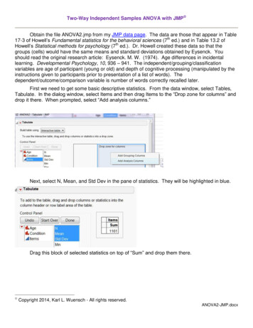
8For simple effects that involve only two groups, you can calculate Cohen’s d, as shown belowfor the main effect of age.There is an alternative method of conducting the tests of the simple main effects. One couldconduct a one-way ANOVA testing the effects of condition using only the data from the youngstersand then do the same using only the data from the oldsters. This would result in one having differenterror terms for the two age groups, but that would be appropriate were there evidence ofheterogeneity of variance between the age groups.Likewise, one could conduct five one-way ANOVAs (or t-tests), each testing the effect of ageat one of the five levels of recall condition.Figure 1Recall in Young and Old ParticipantsMean Items geryIntentionalRecall ConditionLook at the plot above. I created this plot in Microsoft Office. JMP will give you an interactionplot, if you request it, but it is pretty lame. The plot makes it pretty clear that there is an interactionhere. The difference between the oldsters and the youngsters is quite small when the experimentalcondition is one with little depth of cognitive processing (counting or rhyming), but much greater withhigher levels of depth of cognitive processing. With the youngsters, recall performance increaseswith each increase in depth of processing. With the oldsters, there is an interesting dip inperformance in the intentional condition. Perhaps that is a matter of motivation, with oldsters justrefusing to follow instructions that ask them to memorize a silly list of words.The interpretation of the effect of age is straightforward -- the youngsters recalled significantlymore items than did the oldsters, 3.1 items on average. Since there are only two levels of age, wecan use Cohen’s d as the estimate of effect size. The pooled within-age standard deviation iscomputed by taking the square root of the mean of the two groups’ variances --