Transcription
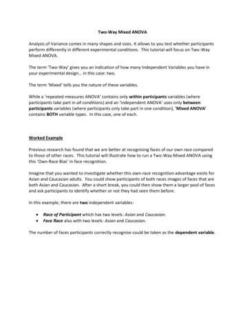
Two-Way Mixed ANOVAAnalysis of Variance comes in many shapes and sizes. It allows to you test whether participantsperform differently in different experimental conditions. This tutorial will focus on Two-WayMixed ANOVA.The term ‘Two-Way’ gives you an indication of how many Independent Variables you have inyour experimental design in this case: two.The term ‘Mixed’ tells you the nature of these variables.While a ‘repeated-measures ANOVA’ contains only within participants variables (whereparticipants take part in all conditions) and an ‘independent ANOVA’ uses only betweenparticipants variables (where participants only take part in one condition), 'Mixed ANOVA'contains BOTH variable types. In this case, one of each.Worked ExamplePrevious research has found that we are better at recognising faces of our own race comparedto those of other races. This tutorial will illustrate how to run a Two-Way Mixed ANOVA usingthis ‘Own-Race Bias’ in face recognition.Imagine that you wanted to investigate whether this own-race recognition advantage exists forAsian and Caucasian adults. You could show participants of both races images of faces that areboth Asian and Caucasian. After a short break, you could then show them a larger pool of facesand ask participants to identify whether or not they had seen them before.In this example, there are two independent variables: Race of Participant which has two levels: Asian and Caucasian. Face Race also with two levels: Asian and Caucasian.The number of faces participants correctly recognise could be taken as the dependent variable.
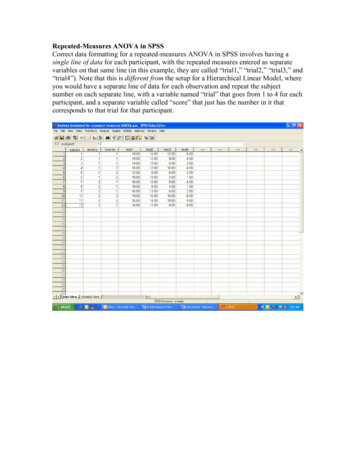
This is what the data collected should look like in SPSS (and can be found in the SPSS file ‘Week3 ORB Data.sav’):As a general rule in SPSS, each row in the spreadsheet should contain all of the data providedby one participant.For within participants variables, separate columns need to represent each of the conditions ofthe experiment (as each participant contributes multiple data points).Between participants variables are coded in a separate column, where the different levels orconditions of the IV refer to separate individuals.The different columns in SPSS display the following data: ID No: This just refers to the ID number assigned to the participants. We use numbersas identifiers instead of participant names, as this allows us to collect data while keepingthe participants anonymous.
Race: This just refers to our between participants variable: participant race. Asparticipants were either one race or the other, codes have been used to tell SPSS whichcondition each of the participants belonged to. In this case:1 Caucasian2 AsianRevisit the tutorial Adding Variables to see how this is done. Asian Face: This column represents one level of our within participants IV: race of face.As participants saw all facial stimuli, conditions are represented by different columns.This column contains the number of faces participants correctly recognised when thefacial stimuli were Asian. Cauc Face: This column represents one level of our within participants IV: race of face.It contains the number of faces participants correctly recognised when the facial stimuliwere Caucasian.We will now walk you through how to run a Mixed ANOVA in SPSSTo start the analysis, begin by CLICKING on the Analyze menu, select the General Linear Modeloption, and then the Repeated Measures. sub-option.You always select this option, whenever you have a within participants variable.
The “Repeated Measures Define Factor(s)” box should now appear. This is where we tell SPSSwhat our within-participants IV is, and how many levels it has.It doesn’t matter what name we give our variable, but it’s probably a good idea to give it asensible name, that we can interpret easily when we look at the output. In this case, let’s nameour variable Face Race (the underscore is used to separate the words, as SPSS doesn't likespaces in variable names).We can define our first variable by typing the name (Face Race) into the Within-Subject FactorName box, and entering the number of levels (2) into the Number of Levels box:CLICK on Add to add this variable to the analysis.Once you have finished defining your IV, CLICK on the Define button to continue with theanalysisThis opens the main ANOVA dialog box.
First, we need to tell SPSS what our between-participants variable is. To do this, SELECT theParticipant Race variable and move it across to the Between-Subjects Factor(s) box byCLICKING on the blue arrow to the left of the box.Next, we need to tell SPSS what the conditions of our within-participants variable are. In theWithin-Subjects Variables box itself, there are a series of question marks with bracketednumbers. These numbers represent the levels of our IVs. Our task is to replace the questionmarks with the names of the conditions that will map onto the variable level codes.To do this, SELECT the two IV conditions: Asian faces and Caucasian faces (when doing thisyourself, hold down the SHIFT key to select multiple options simultaneously). Now add theconditions to the Within-Subjects Variables box by CLICKING on the top arrow button.
Now we have told SPSS what is it that we want to analyse, we are almost ready to run theANOVA. But before we do, we need to ask SPSS to produce some other information for us.First, we want to ask SPSS to produce some descriptive statistics for our different conditions(i.e. means and standard deviations). CLICK on the Options button (highlighted in the imageabove) to do this.This options the Repeated Measures: Opens dialog box. To produce means for the differentvariables and conditions, highlight all of the factor names in the Factor(s) and FactorInteractions box, as is shown here. When doing this yourself, remember that if you hold downthe Shift key you can click on and highlight all of the factors in one go. (OVERALL) just gives youthe overall mean of the whole data set. As we are looking for group differences, this isn't veryinformative. so it isn't really worth including in this step (although you can if you like)!To move the variables across, CLICK the arrow (highlighted above).
In the bottom half of the dialog box, there are a number of tick box options that you can selectto get more information about the data in your output. In this example we are just going toselect three.First, CLICK on Descriptive Statistics, sowe can produce our means and standarddeviations.Next, CLICK on Estimates of effect size toproduce effect size information.Third, whenever you carry out an ANOVAwhich contains a between-participantsvariable, the assumption of homogeneityof variance must be met. This assumesthat the groups you are comparing have asimilar dispersion of scores.To test the assumption, CLICK on theHomogeneity Tests option now.Finally, CLICK on Continue to proceed.Almost there but before we can run the analysis, we need to tell SPSS to produce some morethings for our output. There are a number of other buttons we could select here. If any of ourIVs had more than two levels (or conditions) we would need to select the Post-Hoc testsbutton. But as both Race of Participant and Face Race only have two, we can skip this optionon this occasion. Visit the tutorial on One-Way Independent ANOVA to see more about the PostHoc options available in SPSS.Instead, we next want to tell SPSS to create a graph of our data for us. This will help usinterpret any interaction there might be between the two Independent Variables. CLICK on thePlots button to do this.
Here we are going to tell SPSS what type of graph we want. While it doesn’t really matterwhich way round you put the variables on the graph, it is usually better to put the IV with themost levels on the horizontal axis and the other on as separate lines.In this case both variables have the same number of levels: two. As such, the order reallydoesn’t matter. As Race is already highlighted, start by moving it across to the Horizontal Axisbox using the top blue arrow. Next, SELECT Face Race and move it across to the SeparateLines box using the appropriate arrow.CLICK on the Add button to add it to the Plots box, and then CLICK Continue to proceed.We are now ready to run the analysis!CLICK OK to continue
This opens the Output window, where SPSS produces all of the statistics that you asked for:There is quite a lot of output for Analysis of Variance, but don’t worry - this tutorial will talk youthrough the output you need, box by box.Within-Subjects FactorsThis box is just here to remind you what values you haveassigned the different levels of your within-participantsvariable, and what they mean. You may find it useful torefer back to this when interpreting your output.From looking at the box you should be able to see that forthe first factor, Face Race, there are two levels, where:1 Asian Faces and 2 Caucasian Faces.
Between-Subjects FactorsThis box is just here to remind you whatvalues you have assigned the differentlevels of your between-participantsvariable, and what they mean. You mayfind it useful to refer back to this wheninterpreting your output.From looking at the box you should be able to see that for the second factor, Race, there arealso two levels, where: 1 Caucasian participants and 2 Asian participants.Descriptive StatisticsThis table gives you your descriptive statistics. It’s good to look at and report these, as they cangive you an important insight into the pattern of your data. From this table we can see theaverage (mean) number of faces recognised for each of the possible variable conditions. Youcan also see the variation in the data (i.e. spread of scores) for the different groups from thestandard deviation.From this table we can see that on average, the overall Caucasian and Asian participantsrecognised similar numbers of faces (means 26.70 and 26.75 respectively).However, the breakdown of conditions showed that for the Asian facial stimuli, Asianparticipants got more correct responses (mean 27.60, SD 2.30) than Caucasian participants(mean 25.90, SD 2.34); but for the Caucasian faces, Caucasian participants (mean 27.45,SD 2.21) outperformed the Asian participants (mean 25.95, SD 2.68).Box’s Test of Equality of Covariance Matrices and Multivariate TestsYou only need the next couple of output boxes when you have multiple dependent variables(which we don’t). Skip over these and go straight to the Mauchly’s Test of Sphericity box.
Mauchly's Test of SphericityThis table tests whether the assumption of sphericity has been met. This is a bit like theassumption of homogeneity of variance for independent tests; and like Levene's test, we do notwant Mauchly's test to be significant. However, rather than assuming equal levels of variancein the data for the different conditions, in this case we assume that the relationship betweenthe different pairs of conditions is similar.The good news is, you only need to look at this table when you have a within participantsvariable with more than two levels (i.e. more than one pair). which in this case, we don't have- Face Race only has two conditions!!Tests of Within-Subjects EffectsThis is the one of the most important tables in the output. It gives you the ANOVA results foryour within-participants variable (Face Race); and any interactions with that variable.
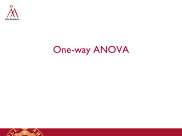
The key columns you need to interpret your analysis are: df stands for degrees of freedom. Degrees of freedom are crucial in calculatingstatistical significance, so we need to report them. For each main effect and interactionthere are two df values of interest: the factor (or interaction) df and the error term df.In this example the dfs can be found in the Sphericity Assumed rows (you would onlyuse the other rows if the sphericity assumption had not been met). F stands for F-Ratio. This column gives you the F-Ratio statistics calculated by theANOVA. It is essentially calculated by dividing the systematic variance (i.e. the variationin your data that can be explained by your experimental manipulation) by theunexpected, unsystematic variance. The larger your F-Ratio, the more likely it is thatyour experimental manipulation (your IV) will have had a significant effect on the DV.In this example the you need to report the values in the Sphericity Assumed rows. Sig stands for Significance Level. This column gives you the probability that the resultscould have occurred by chance if the null hypothesis were true. The p-value should besmaller than 0.05 for the F-ratio to be significant. If this is the case (i.e. p .05) we rejectthe null hypothesis and infer that our experimental manipulation (our IV) has had asignificant effect.However, if the p-value is larger than 0.05, we have to retain the null hypothesis: thatthere is no difference between the conditions (or no interaction). Partial Eta Squared. While the p-value can tell you whether your main effects andinteraction terms are statistically significant, partial eta squared (ηp2) tells you about themagnitude of these effects. As such, we refer to this as a measure of effect size. Tointerpret your effects sizes, you can use the following cut-offs:o 0.14 or more are large effectso 0.06 or more are medium effectso 0.01 or more are small effectsSo we know which columns we need to look at, but what numbers do we use?Which row you choose depends on whether your assumption of Sphericity has been met. Ifyour Mauchley’s test was non-significant (i.e. the assumption had been met), or if you have lessthan 3 levels in your within-participants IV (which we do!), then you read across from theSphericity Assumed row. If Mauchley’s had been significant, then you would need to use oneof the other rows.SPSS groups your analysis into blocks: one block for each variable and interaction.
First, let’s look at Face Race.Using the Sphericity Assumed row, you need to report your results as:F (IV df, error df) F-Ratio, p Sig, ηp2 Partial Eta Squared.along with a sentence, explaining what you have found. In this case you might say:There was no significant main effect of Face Race on face recognition scores overall(F(1, 38) .01, p .92, ηp2 .001).Next, we can use the same method to look at the interaction term. The results are in theFace Race * Race block. Again, using the Sphericity Assumed row to locate the correct values,you might report your results as something like:There was a significant interaction between Face Race and Race in terms of recognitionscores (F(1, 38) 10.59, p .002, ηp2 .22).Tests of Within-Subjects ContrastsYou really don't need to worry about this table for interpreting your results. so skip over thisand go straight to your Levene’s Test of Equality of Error Variances which assesses theassumption of homogeneity of variance for your between-participants variable (Race).
Levene's Test of Equality of Error VariancesWhen conducting an ANOVA with any between-participants variables, one assumption thatmust be met is that the groups you are comparing have a similar dispersion of scores (i.e.homogeneity of variance). The Levene’s Statistic tells us whether or not this is the case.For Mixed ANOVA, this assumption is assessed at all levels of your within-participants variable(i.e. for both Asian and Caucasian facial stimuli).If the test is significant this indicates that there are statistically significant differences in the wayin the data are dispersed, suggesting that the assumption has been violated. As such, we arelooking for a non-significant result here. In this example, the Sig. column tells us that this iswhat we have found as both p-values are greater than .05.Tests of Between-Subjects EffectsThis is another one of the most important tables in the output. This is where we get ourANOVA statistics for the between-participants variable (Race).As with the Tests of Within-Subjects Effects table, the columns we need to interpret youranalysis are highlighted above: df, F, Sig and Partial Eta SquaredIn this case we need to read across the row representing our IV (labelled Race) and the Errorrow.
As with the results for the within-participants variables and interaction, you need to report yourresults using the following formula:F (IV df, error df) F-Ratio, p Sig, ηp2 Partial Eta Squared.along with a sentence, explaining what you have found. For example:There was no significant main effect of Race on face recognition scores overall(F(1, 38) .03, p .86, ηp2 .001).We now have our ANOVA results for both of our IVs (Face Race and Race) and the interactionbetween these variables. But the question is, what does it all mean?We know that while neither of our IVs produced a significant main effect, we did find aninteraction between our IVs. but we now need to interpret and explain what this actuallymeans in English!! To do that, we need to refer back to our Descriptive Statistics to see what ishappening in each of our different conditions.Estimated Marginal MeansThese boxes show you the breakdown of the means for the different levels of your IVs, and allof the different condition combinations. For a Mixed ANOVA, the mean values are the same asthose displayed the Descriptive Statistics box at the beginning of your output. Note that theseboxes report the Standard Error rather than the Standard Deviation through.This first box tells you the overall mean recognition scores for both levels of your first IV:Participant Race. Here we can see that both Caucasian (mean 26.68) and Asian (mean 26.78) participants performed similarly.
The second box tells you the overall mean recognition scores for the levels of your second IV:Face Race. From the very first box in the SPSS output, we saw that 1 Asian Faces and2 Caucasian Faces.As such, we can see that overall participants performed similarly for both Asian (mean 26.75)and Caucasian (mean 26.70) faces.The final box gives you the breakdown of facial recognition scores for all of your conditioncombinations. This can help you to interpret your interaction. Again, remembering that thenumber codes are 1 Asian Faces and 2 Caucasian Faces, we can interpret the pattern of resultsaccordingly.Here we can see that while Asian participants recognised more Asian faces (mean 27.60) thanCaucasian faces (mean 29.95); Caucasian participants showed the opposite pattern (Asianfaces mean 25.90; Caucasian faces mean 27.45), suggestive of an own-race bias in facerecognition.Profile PlotsThe final part of the output is the Profile Plot. Graphs can be really useful in helping you tovisualise and understand your interaction. When looking at the graph, it may help you toconsider the following:
Are the lines doing the same thing. If not, what are they doing? Are some points on the graph closer together than others?Here, the blue line represents Face Race 1 Asian Faces. From the way the line slopes we cansee that Asian Participants performed much better for this stimuli than Caucasian Participants.In contrast, the green line (which represents Face Race 2 Caucasian Faces) slopes in theopposite direction. For this stimuli type, Caucasian participants performed better AsianParticipants.As well as looking at the slopes of the lines, we can also look at the vertical distance betweenthe dots for each race of participant. Doing this we can see that both races performed betterfor faces of their own race, compared to those of the other race. And this own-race advantagewas of a similar magnitude in both cases.The trick now is to put all of the information from your output together to make a resultssection that is sensible and meaningful!!
How do we write up our results?When writing up the findings from your analysis in APA format, you need to include all of therelevant information covered by the previous slides. What were the inferential statistics for your IVso i.e. what were the ANOVA results For significant findings, where did the significant difference(s) lieo i.e. what were the results of your post hoc tests, if you did them What was the pattern and direction of these differenceso i.e. what were the means and descriptive statistics for your conditions If the interaction term was significant, what does it mean in Englisho i.e. describe what was happening in the different conditionsIt is usually helpful to the reader of your results if you include a table of the means andstandard deviations for all of the conditions in your results. It also helps to include a graph ofyour results. You can edit your graph by double clicking on it in the output in SPSS.For this example, you might end up writing a results section that looks a bit like this:The results of the Two-Way Mixed ANOVA showed that there was no significant maineffect of Participant Race (F(1, 38) .03, p .86, ηp2 .001) on face recognition scores,with Caucasian (mean 26.68) and Asian (mean 26.78) performing similarly overall.In addition, there was also no significant main effect of Face Race on recognitionscores (F(1, 38) .01, p .92, ηp2 .001), with participants showing similar averagerecognition scores for Asian (mean 26.75) and Caucasian (mean 26.70) faces.In contrast, there was a significant interaction between Race of Participant and FaceRace (F(1, 38) 10.59, p .002, ηp2 .22). Descriptive statistics showed that whileAsian participants performed better for Asian facial stimuli (mean 27.60, SD 2.30)compared to Caucasian stimuli (mean 25.95, SD 2.68); Caucasian participantsshowed the opposite pattern (Asian faces mean 25.90, SD 2.34; Caucasian facesmean 27.45, SD 2.21). From looking at the graph we can see that both racesshowed a similarly sized recognition advantage for own-race faces.These findings support the notion of an own-race bias in face recognition.This brings us to the end of this tutorial. Why not download the data file used in this tutorialand see if you can run the analysis yourself?
on this occasion. Visit the tutorial on One-Way Independent ANOVA to see more about the Post Hoc options available in SPSS. Instead, we next want to tell SPSS to create a graph of our data for us. This will help us interpret any interaction there might be between the two Independent Variables. CLICK on the Plots button to do this.