Transcription
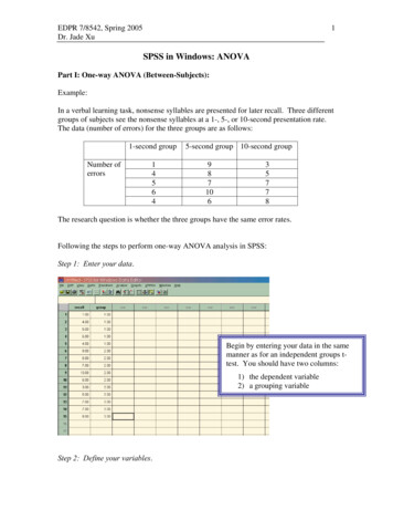
EDPR 7/8542, Spring 2005Dr. Jade Xu1SPSS in Windows: ANOVAPart I: One-way ANOVA (Between-Subjects):Example:In a verbal learning task, nonsense syllables are presented for later recall. Three differentgroups of subjects see the nonsense syllables at a 1-, 5-, or 10-second presentation rate.The data (number of errors) for the three groups are as follows:1-second groupNumber oferrors145645-second group 10-second group98710635778The research question is whether the three groups have the same error rates.Following the steps to perform one-way ANOVA analysis in SPSS:Step 1: Enter your data.Begin by entering your data in the samemanner as for an independent groups ttest. You should have two columns:1) the dependent variable2) a grouping variableStep 2: Define your variables.
EDPR 7/8542, Spring 2005Dr. Jade Xu2Remember that to do this, you can simply double-click at the top of the variable’scolumn, and the screen will change from “data view” to “variable view,” prompting youto enter properties of the variable. For your dependent variable, giving the variable aname and a label is sufficient. For your independent variable (the grouping variable), youwill also want to have value labels identifying what numbers correspond with whichgroups. See the following figure for how to do this.Start by clicking on thecell for the “values” forthe variable you want.The dialog box belowwill appear.Remember to click the“Add” button each time you entera value label; otherwise,the labels will not be added toyour variable’s properties.
EDPR 7/8542, Spring 2005Dr. Jade Xu3Step 3: Select Oneway ANOVA from the command list in the menu as follows:Note: There is more than one way to run ANOVA analysis in SPSS. For now, theeasiest way to do it is to go through the “compare means” option. However, since theanalysis of variance procedure is based on the general linear model, you could also usethe analyze/general linear model option to run the ANOVA. This command allows forthe analysis of much, much more sophisticated experimental designs than the one wehave here, but using it on these data would yield the same result as the One-way ANOVAcommand.
EDPR 7/8542, Spring 2005Dr. Jade Xu4Step 4: Run your analysis in SPSS.Once you’ve selected the One-way ANOVA, you will get a dialog box like the one at thetop. Select your dependent and grouping variables (notice that unlike in the independentsamples t-test, you do not need to define your groups—SPSS assumes that you willinclude all groups in the analysis.While you’re here, you might as wellselect the “options ” button, and checkthat you would like descriptive and HOVstatistics. Another thing you might needis the Post Hoc tests. You can also selectfor SPSS to plot the means if you like.
EDPR 7/8542, Spring 2005Dr. Jade Xu5Step 5: View and interpret your output.Note that the descriptive statistics includeConfidence Intervals, your test ofhomogeneity of variance is in a separatetable from your descriptive, and yourANOVA partitions your sum of squares.If you wish to do this with syntax commands, you can see what the syntax looks like byselecting “paste” when you are in the One-way ANOVA dialog box.Step 6: Post-hoc testsOnce you have determined that differences exist among the group means, post hocpairwise and multiple comparisons can determine which means differ. SPSS presentsseveral choices, but different post hoc tests vary in their level by which they control TypeI error. Furthermore, some tests are more appropriate than other based on theorganization of one's data. The following information focuses on choosing anappropriate test by comparing the tests.
EDPR 7/8542, Spring 2005Dr. Jade Xu6A summary leading up to using a Post Hoc (multiple comparisons):Step 1. Test homogeneity of variance using the Levene statistic in SPSS.a. If the test statistic's significance is greater than 0.05, one may assume equalvariances.b. Otherwise, one may not assume equal variances.Step 2. If you can assume equal variances, the F statistic is used to test the hypothesis. Ifthe test statistic's significance is below the desired alpha (typically, alpha 0.05),then at least one group is significantly different from another group.Step 3. Once you have determined that differences exist among the means, post hocpairwise and multiple comparisons can be used to determine which means differ.Pairwise multiple comparisons test the difference between each pair of means,and yield a matrix where asterisks indicate significantly different group means atan alpha level of 0.05.Step 4. Choose an appropriate post hoc test:a. Unequal Group Sizes: Whenever you violate the equal n assumption for groups,select any of the following post hoc procedures in SPSS: LSD, Games-Howell,Dunnett's T3, Scheffé, and Dunnett's C.b. Unequal Variances: Whenever you violate the equal variance assumption forgroups (i.e., the homogeneity of variance assumption), check any of the followingpost hoc procedures in SPSS: Tamhane’s T2, Games-Howell, Dunnett's T3, andDunnett's C.
EDPR 7/8542, Spring 2005Dr. Jade Xu7c. Selecting from some of the more popular post hoc tests: Fisher's LSD (Least Significant Different): This test is the most liberal of allPost Hoc tests and its critical t for significance is not affected by the numberof groups. This test is appropriate when you have 3 means to compare. Itis not appropriate for additional means. Bonferroni (AKA, Dunn’s Bonferroni): This test does not require the overallANOVA to be significant. It is appropriate when the number ofcomparisons (c number of comparisons k(k-1))/2) exceeds the numberof degrees of freedom (df) between groups (df k-1). This test is veryconservative and its power quickly declines as the c increases. A good rule ofthumb is that the number of comparisons (c) be no larger than the degrees offreedom (df). Newman-Keuls: If there is more than one true null hypothesis in a set ofmeans, this test will overestimate they familywise error rate. It isappropriate to use this test when the number of comparisons exceeds thenumber of degrees of freedom (df) between groups (df k-1) and one doesnot wish to be as conservative as the Bonferroni. Tukey's HSD (Honestly Significant Difference): This test is perhaps the mostpopular post hoc. It reduces Type I error at the expense of Power. It isappropriate to use this test when one desires all the possible comparisonsbetween a large set of means (6 or more means). Tukey's b (AKA, Tukey’s WSD (Wholly Significant Difference)): This teststrikes a balance between the Newman-Keuls and Tukey's more conservativeHSD regarding Type I error and Power. Tukey's b is appropriate to usewhen one is making more than k-1 comparisons, yet fewer than (k(k-1))/2comparisons, and needs more control of Type I error than NewmanKuels. Scheffé: This test is the most conservative of all post hoc tests. Compared toTukey's HSD, Scheffé has less Power when making pairwise (simple)comparisons, but more Power when making complex comparisons. It isappropriate to use Scheffé's test only when making many post hoccomplex comparisons (e.g. more than k-1).End note:Try to understand every piece of information presented in the output. Button-clicks inSPSS are not hard, but as an expert, you are expected to explain the tables and figuresusing the knowledge you have learned in class.
EDPR 7/8542, Spring 2005Dr. Jade Xu8Part II: Two-way ANOVA (Between-Subjects):Example:A researcher is interested in investigating the hypotheses that college achievement isaffected by (1) home-schooling vs. public schooling, (2) growing up in a dual-parentfamily vs. a single-parent family, and (3) the interaction of schooling and family type.She locates 5 people that match the requirements of each cell in the 2 2 (schooling family type) factorial design, like this:SchoolingHome PublicFamily type Dual ParentSingle ParentAgain, we’ll do the 5 steps of hypothesis testing for each F-test. Because step 5 can beaddressed for all three hypotheses in one fell swoop using SPSS, that will come last.Here are the first 4 steps for each hypothesis:A. The main effect of schooling type1.;2. F3. N 20; F(1,16)4.,B. The main effect of family type;1.2. F3. N 20; F(1,16)4.,C. The interaction effect1.2. F3. N 20; F(1,16)4.;Step 5, using SPSS;
EDPR 7/8542, Spring 2005Dr. Jade XuFollowing the steps to perform two-way ANOVA analysis in SPSS:Step 1: Enter your data.Because there are two factors, there are now two columns for "group": one for familytype (1: dual-parent; 2: single-parent) and one for schooling type (1: home; 2: public).Achievement is placed in the third column. Note: if we had more than two factors, wewould have more than two group columns. See how that works? Also, if we had morethan 2 levels in a given factor, we would use 1, 2, 3 (etc.) to denote level.Step 2. Choose Analyze - General Linear Model - Univariate.9
EDPR 7/8542, Spring 2005Dr. Jade Xu10Step 3. When you see a pop-up window like this one below, plop Fmly type andSchooling into the "Fixed Factors" window and Achieve into the "Dependent Variable"window.In this window, you might as wellselect the “options ” button, andcheck that you would like descriptiveand HOV statistics. Another thing youmight need is the Post Hoc tests. Youcan also select for SPSS to plot themeans if you like.and click on "OK," yielding:Tests of Between-Subjects EffectsDependent Variable: AchieveSourceCorrected ModelType III Sumof Squares1.019(a)3Mean Square.3404.46514.465548.204.000Fmly Fmly type * 61420Corrected Total1.14919InterceptdfF41.705Sig.000a R Squared .887 (Adjusted R Squared .865)I have highlighted the important parts of the summary table. As with the one-wayANOVA, MS SS/df and F MSeffect / MSerror for each effect of interest. Also, valuesadd up to the numbers in the "Corrected Total" row.An effect is significant if p α or, equivalently, if Fobs / Fcrit. The beauty of SPSS is thatwe don't have to look up a Fcrit if we know p. Because p α for each of the three effects(two main effects and one interaction), all three are statistically significant.One way to plot the means (I used SPSS for this – the "Plots" option in the ANOVAdialog window) is:
EDPR 7/8542, Spring 2005Dr. Jade XuThe two main effects and interaction effect are very clear in this plot. It would be verygood practice to conduct this factorial ANOVA by hand and see that the results matchwhat you get from SPSS.Here is the hand calculatioin. First, degrees of freedom.Note that these df match those in the ANOVA summary table.Next, the means.11
EDPR 7/8542, Spring 2005Dr. Jade XuThen, sums of squares.and by subtraction for the remaining ones:Note that these sums of squares match those in the ANOVA summary table. So the Fvalues are:12
EDPR 7/8542, Spring 2005Dr. Jade Xu13Note that these F values are within rounding error of those in the ANOVA summarytable.According to Table C.3 (because α .05 ), the critical value for all three F-tests is 4.49.All three Fs exceed this critical value, so we have evidence for a main effect of familytype, a main effect of schooling type, and the interaction of family type and schoolingtype. This agrees with our intuition based on the mean plots.In the current example, a good way to organize the data is :Dual ParentMean(1j)Single ParentMean(2j)Mean(j)SchoolingHome Public 32 0.208 0.8320.5200.320 0.625 0.4725Note: Post-hoc testsOnce you have determined that differences exist among the group means, post hocmultiple comparisons can determine which means differ.
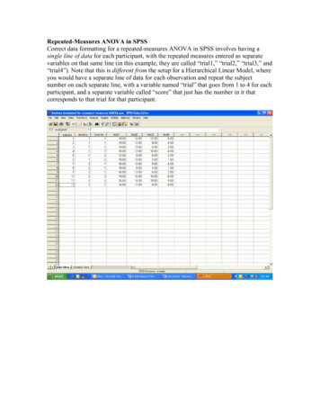
EDPR 7/8542, Spring 2005Dr. Jade Xu14Part III: One-way Repeated Measures ANOVA (Within-Subjects):The LogicJust as there is a repeated measures or dependent samples version of the Student t test,there is a repeated measures version of ANOVA. Repeated measures ANOVA followsthe logic of univariate ANOVA to a large extent. As the same participants appear in allconditions of the experiment, however, we are able to allocate more of the variance. Inunivariate ANOVA we partition the variance into that caused by differences withingroups and that caused by differences between groups, and then compare their ratio. Inrepeated measure ANOVA we can calculate the individual variability of participants asthe same people take part in each condition. Thus we can partition more of the error (orwithin condition) variance. The variance caused by differences between individuals isnot helpful when deciding whether there is a difference between occasions. If we cancalculate it we can subtract it from the error variance and then compare the ratio of errorvariance to that caused by changes in the independent variable between occasions. Sorepeated measures allows us to compare the variance caused by the independent variableto a more accurate error term which has had the variance caused by differences inindividuals removed from it. This increases the power of the analysis and means thatfewer participants are needed to have adequate power.The ModelFor the sake of simplicity, I will demonstrate the analysis by using the following threeparticipants that were measured in four occasions.ParticipantOccasion 1Occasion 2Occasion 3Occasion 417755 2426653 2035443 16 18 17 14 11SPSS AnalysisStep 1: Enter the data
EDPR 7/8542, Spring 2005Dr. Jade Xu15When you enter the data remember that it consists of three participants measured on fouroccasions and each row is for a separate participant. Thus, for this data you have threerows and four variables, one for each occasion.Step 2. To perform a repeated measures ANOVA you need to go through Analyze toGeneral Linear Model, which is where you found one of the ways to perform UnivariateANOVA. This time, however, you click on Repeated Measures.After this the followingdialogue box should appear.The dialogue box refers to the occasions as awithin subjects factor and it automaticallylabels it factor 1. You can if you want giveit a different name one which has meaningfor the particular data set you are looking at.Although SPSS knows that there is a withinsubjects factor, it does not know how many levels of it there are, in other words it doesnot know how many occasions you tested you subjects. Here you need to type in 4 thenclick on the Add button and then the Define button, which will let you tell SPSS whichoccasions you want to compare. If you do this the following dialogue box will appear.
EDPR 7/8542, Spring 2005Dr. Jade Xu16Next we need to put the variables into the within subjects box; as you can see we havealready put occasion 1 in slot (1) and occasion 2 in slot (2). We could also ask for somedescriptive statistics by going to Options and selecting Descriptives, once this is donepress OK and the following output should appear.General Linear ModelWithin-Subjects FactorsMeasure: MEASURE AS4This first box just tellsus what the variables are
EDPR 7/8542, Spring 2005Dr. Jade Xu17Descriptive StatisticsMean6.00005.66674.66673.6667occasion 1occasion 2occasion 3occasion 4Std. Deviation1.00001.5275.57741.1547NFrom the descriptives, it isclear that the means getsmaller over occasions. Thebox below should be ignored.3333Multivariate TestsbEffectFACTOR1ValueF.a.a.a.aPillai's TraceWilks' LambdaHotelling's TraceRoy's Largest Root.Hypothesis df.Error dfSig.a. Cannot produce multivariate test statistics because of insufficient residual degrees offreedom.b.Design: InterceptWithin Subjects Design: FACTOR1Mauchly's Test of SphericitybMeasure: MEASURE 1EpsilonWithin Subjects EffectFACTOR1Mauchly's 667aHuynh-Feldt.Lower-bound.333Tests the null hypothesis that the error covariance matrix of the orthonormalized transformed dependent variables isproportional to an identity matrix.a. May be used to adjust the degrees of freedom for the averaged tests of significance. Corrected tests are displayed in theTests of Within-Subjects Effects table.b.Design: InterceptWithin Subjects Design: FACTOR1This box gives a measure of sphericity. Sphericity is similar to the assumption ofhomogeneity of variances in Univariate ANOVA. It is a measure of thehomogeneity of the variances of the differences between levels. That is in this casethat the variance of the difference between occasion 1 and 2 is similar to thatbetween 3 and 4 and so on. Another way to think of it is that it means thatparticipants are performing in similar ways across the occasions. If the Mauchly teststatistic is not significant then we use the sphericity assumed F value in the next box.If it is significant then we should use the Greenhouse-Geisser corrected F value. Inthis case there are insufficient participants to calculate Mauchly. Try adding onemore participant who scores four on every occasion and check the sphericity.
EDPR 7/8542, Spring 2005Dr. Jade Xu18Tests of Within-Subjects EffectsMeasure: MEASURE 1SourceFACTOR1Error(FACTOR1)Sphericity ericity e III Sumof 0df32.000.1.00064.000.2.000Mean .10.000Sig.009.028.087This is the most important box for repeated measures ANOVA. As you can see the Fvalue is 10.Tests of Within-Subjects ContrastsMeasure: MEASURE CubicLinearQuadraticCubicType III Sumof Squares9.600.3336.667E-02.400.667.933df111222Mean 43Sig.020.423.742The Within-Subjects contrast box test for significant trends. In this case there is asignificant linear trend, which means in this case there is a tendency for the data to fall ona straight line. In other words the mean for occasion 1 is larger than occasion 2 which islarger than occasion 3 which is larger than occasion 4. If we have a quadratic trend wewould have an inverted U or a U shaped pattern. It is important to remember that thisbox is only of interest if the overall F value is significant and that it is a test of a trend nota specific test of differences between occasions. For that we need to look at post hoctests.Hand Calculation:It would be very good practice to conduct this repeated-measures ANOVA by hand andsee that the results match what you get from SPSS. The only formula needed is theformula for the sum of squares that we used for univariate ANOVA; x2 - ( x )2/n.
EDPR 7/8542, Spring 2005Dr. Jade Xu19The first step is to calculate the total variability or the total sum of squares (SST). It willnot surprise you to learn that this is the same as you were doing a univariate ANOVA.That is, (49 49 25 25 36 36 25 9 25 16 16 9) - (60)2/12 320 - 300 20.We now calculate the variability due to occasions. This variability is calculated exactlythe same way as the within group variability is calculated for a univariate ANOVA. Sofor this data the variability due to occasions is the sum of the variability within eachoccasion.The variability for occasion 1 is (49 36 25) - (18)2 /3; for occasion 2 it is (49 36 16) 172/3. See if you can work out the sum for occasions 3 and 4. The answers shouldcome to occasion 3 0.66 and occasion 4 2.66 and added to occasion 1 and 2, we get asum of 10. Again this is no surprise as it should be the same for within group variabilityfor a univariate ANOVA. This time, however, this variability is very important as it isnot a measure of error but a measure of the effect of the independent variable, as theparticipants have remained the same but the independent variable has altered with theoccasion.We now need to calculate the variation caused by individual variability, that is the threeparticipants in this study differ in their overall measures here. This calculation issomething we have not met in univariate ANOVA but the principles remain the same.Looking at the data you can see that overall participant 1 had the highest score of 24,participant 2 had an overall score of 20 and participant 3 had an overall score of 16.To calculate individual variability we still use the sum of squares formula x2 - ( x )2/n.In this case we get (242 202 162) - (60)2/3 (576 400 256)-3600/3 32.Alarm bells may be ringing as you will see that we have more variability than the total.However, we have not adjusted this figure for the number of occasions; to do that wedivide in this instance by 4 to get a figure of 8. So the variability that is caused bydifferences in participants is 8.Another way to calculate the individual variability is to divide the squared row totals bythe number of occasions and then subtract the correction factor. This would give us;242/4 202/4 162/4 308, and then subtracting the correction factor gives us 308-300 8.At this stage we have calculated all of the variabilities that we need to perform ouranalysis; the variability due to occasions that is caused by the differences in theindependent variable across occasions is 10, the variability due to differences inindividuals is 8 and the residual variability is 2. The residual or error variability is thetotal variability (20) minus the sum of the variability due to occasions and individuals(18).The next step is to calculate the degrees of freedom so that we can turn these variabilitiesinto variances or mean squares (MS). The total degrees of freedom is 12 -1 11, as inthe univariate ANOVA. The degrees of freedom for individuals is the number ofparticipants minus 1, in this case 3 -1 2 and for occasions it is the number of occasions
EDPR 7/8542, Spring 2005Dr. Jade Xu20minus 1, in this case 4-1 3. The residual degrees of freedom is the total minus the sumof the degrees of freedom from individuals and occasions; 11-5 6.The mean squares are then calculated by dividing the variability by the degrees offreedom. The mean square for individuals is 8/2 4, for occasions 10/3 3.33 and for theresidual 2/6 0.33.To calculate the F statistic it is important to remember that we are not interested in theindividual variability of subjects. This is part of the error variance which we cannotcontrol for in a univariate ANOVA, but which we can measure in a repeated measuresdesign and then discard. What we are concerned with is whether our independentvariable which changes on different occasions has an effect on subject's performance.The F ratio we are interested in is, therefore, MSoccasions / MSresidual; 3.33/0.33 which is 10.If you were calculating statistics by hand you would now need to go to a table of valuesfor Fcrit to work out whether it is significant or not. We won't do that we will justperform the same calculation by SPSS and check the significance there.Notes:1. The information presented in this handout is modified from the following websites:For one-way between-subjects rial2.docFor two-way between-subjects ANOVAhttp://www.unc.edu/ preacher/30/anova spss.pdfFor post-hoc tests:http://staff.harrisonburg.k12.va.us/ gcorder/test post hocs.htmlFor repeated-measures /RepeatedmeasuresANOVA.htm2. Other useful web resources ttp://www.oswego.edu/ ept/psych/SPSS/SPSS1wANOVA.html
Step 4: Run your analysis in SPSS. Once you’ve selected the One-way ANOVA, you will get a dialog box like the one at the top. Select your dependent and grouping variables (notice that unlike in the independent samples t-test, you do not need to define your groups—SPSS