WIXLIB

Repeated-Measures ANOVA in SPSSCorrect data formatting for a repeated-measures ANOVA in SPSS involves having asingle line of data for each participant, with the repeated measures entered as separatevariables on that same line (in this example, they are called “trial1,” “trial2,” “trial3,” and“trial4”). Note that this is different from the setup for a Hierarchical Linear Model, whereyou would have a separate line of data for each observation and repeat the subjectnumber on each separate line, with a variable named “trial” that goes from 1 to 4 for eachparticipant, and a separate variable called “score” that just has the number in it thatcorresponds to that trial for that participant.

The procedure is found under “Analyze”/“General Linear Model”/“Repeated Measures.”Use the first pop-up dialog box to define your repeated-measures factor – this is how youtell SPSS that the four different “trial” variables are really all a single person’s scoresover time on one variable. Give your variable a name (like “trial”), and specify howmany different levels it has (i.e., how many times the observation was repeated). Be sureto then hit the “Add” button so that the new variable appears on a list. You can createmultiple repeated-measures variables at this step if you need to. Then click on “Define.”

Select the columns in your dataset that represent the various levels of the repeatedmeasures variable, and use the arrow button to move them into the “blanks” in the righthand column.Next, specify your model. The within-subjects factors represent scores on the DV at eachtrial. Therefore, they will be treated as the dependent (criterion) variable for this analysis.For predictors, enter grouping variables (e.g., treatment vs. control) as “between-subjectsfactors,” and other interval/ratio-level predictors as “covariates.” In this example,participants’ anxiety level (“Anxiety”) and tension level (“Tension”) were bothmanipulated experimentally, so these are entered as grouping variables (“betweensubjects factors”). Therefore, this is a 2 (two levels of anxiety) x 2 (two levels of tension)factorial repeated-measures ANOVA design.

Use the “Options” button to open this window, and click on the check-box to select“Homogeneity Tests.” This will allow you to test the homogeneity of varianceassumption for the repeated-measures dependent variable. This window also shows youall the different interactions that will be tested as part of your analysis. If you don’t wantall of these results, you can select just specific main effects and interactions by using the“Model” button in the main dialog window. Click “Continue” to go on.

One other type of output you might want is a graph showing the average change in scoreson the dependent variable for individuals over time, maybe with the results sorted basedon the experimental group the person is in. The “Plots” button on the main dialog box letsyou do this. In this dialog box, the DV (repeated-measures variable) goes on the“horizontal axis” of the graph. If you just want to see that variable’s change over time,just enter that for the horizontal axis and leave the other fields blank. If you want to seeseparate lines on the graph for people in different groups, put the grouping variable intothe “separate lines” box. Remember to hit the “Add” button to add your graph to the listthat SPSS will provide.Now return to the main dialog box and hit “OK” to see the output.SPSS uses a multivariate analysis to detect repeated-measures effects. This approachassumes that there is some change from each time period to the next on the repeatedmeasure. If you expect more of a “stepwise” pattern in your results, it may be advisableto test only the pre-post difference in the repeated measure. Alternately, you may want toconsider using a different procedure like ANCOVA or HLM.

Here are the results of the multivariate test:Multivariate TestsbEffecttrialtrial * anxietytrial * tensiontrial * anxiety * tensionPillai's TraceWilks' LambdaHotelling's TraceRoy's Largest RootPillai's TraceWilks' LambdaHotelling's TraceRoy's Largest RootPillai's TraceWilks' LambdaHotelling's TraceRoy's Largest RootPillai's TraceWilks' LambdaHotelling's TraceRoy's Largest 9.3611.7731.773.672.3282.0502.050FHypothesis 000a4.0993.0004.099a3.000a4.0993.000Error . Exact statisticb.Design: Intercept anxiety tension anxiety * tensionWithin Subjects Design: trialThe significant p-values show an effect of time (trial) on the dependent variable – awithin-subjects effect reflected by the repeated measures. All four multivariate tests alsoshow a significant interaction between trial and anxiety level, meaning that the level ofanxiety induced in the participant had a significant effect on their performance over time.The effect of tension, by contrast, did not reach conventional levels of statisticalsignificance. Because tension had a non-significant effect, it probably doesn’t make senseto look at the results for the three-way interaction between tension, anxiety, and time.

Next is a test for the assumption of sphericity, which is important in multivariate tests.Mauchly's Test of Sphericity bMeasure: MEASURE 1EpsilonWithin Subjects EffecttrialMauchly's eisser.536aHuynh-Feldt.902Lower-bound.333Tests the null hypothesis that the error covariance matrix of the orthonormalized transformed dependent variables isproportional to an identity matrix.a. May be used to adjust the degrees of freedom for the averaged tests of significance. Corrected tests are displayed inthe Tests of Within-Subjects Effects table.b.Design: Intercept anxiety tension anxiety * tensionWithin Subjects Design: trialIn this case, the assumption of sphericity was not met (because the p-value of the test wassignificant, indicating a significant difference from the conditions under which theassumption holds true). Unfortunately, this means that we cannot rely on the multivariatetests examined above. The “epsilon” values on the right-hand side of this table are threedifferent ways to calculate an appropriate adjustment to the degrees of freedom of the Ftest. The next table shows revised results using each of these corrections. The LowerBound test is the most conservative; the Huynh-Feldt test is generally least conservative.

Tests of Within-Subjects EffectsMeasure: MEASURE 1Sourcetrialtrial * anxietytrial * tensiontrial * anxiety * tensionError(trial)Sphericity ericity ericity ericity ericity e III Sumof 821.6558.000Mean 1.955The revised tests: This time, there is a significant effect of time (trial), but no interactionwith either of the experimental 197.169.209.148.185.155.200

SPSS also automatically tests for nonlinear trends. This can be helpful if you think that aneffect will be curvilinear with respect to time (for example, you might expect an effectstrong at first, diminishing over time). This table shows the same significant linear effectof time on the DV as we saw in the previous analyses, plus a possible quadratic effect forthe interaction between anxiety and time. This effect should be interpreted cautiouslygiven the overall nonsignificant effect of anxiety and the fact that it only barely achievedthe .05 cut-off for significance. Nevertheless, it may be worth further investigation.Tests of Within-Subjects ContrastsMeasure: MEASURE 1Sourcetrialtrial * anxietytrial * tensiontrial * anxiety * ubicLinearQuadraticCubicType III Sumof 8Mean 2.335.535.253.033.144.843.126.159.692.057SPSS concludes the analysis with a univariate test, looking at the main effect of eachpredictor on the average of the four time intervals for the DV. I don’t recommend usingthis particular analysis, as it by definition ignores effects of time. If you really didn’texpect changes over time, you probably wouldn’t have used a repeated-measuresANOVA. But, this analysis may help you to see if there are any main effects of your IVson your DV, if time did not have a significant effect in the analyses examined previously.If you found nonsignificant effects for time, this could at least help to suggest alternativeanalytic strategies for further research.

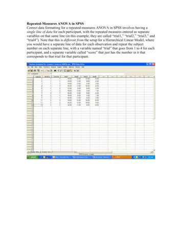
Finally, we have the graphs that were specified in the “Plots” command. These clearlyshow the change over time (trial) in the DV. They also show the hint of a nonlinear effectof anxiety, as there are slight differences between the two anxiety groups on the type ofchange observed in the DV—you can see how the two groups seem to diverge at Trial 4.Again, this is not a firm conclusion (unless that was the effect we expected and that wewere specifically testing for), but it might be worth further investigation.Estimated Marginal Means of MEASURE 118Estimated Marginal Means161412108641234trialEstimated Marginal Means of MEASURE 1Anxiety17.5012Estimated Marginal Means15.0012.5010.007.505.002.50123trial4

Repeated-Measures ANOVA in SPSS Correct data formatting for a repeated-measures ANOVA in SPSS involves having a single line of data for each participant, with the repeated measures entered as separate variables on that same line (in this example, the