Transcription
Types of Statistical TestsDR. MIKE MARRAPODI
Tests t tests ANOVA Correlation Regression Multivariate Techniques Non-parametric
t tests One sample t test Independent t test Paired sample t test
One sample t test Measures: Mean of a single variable When to use: Comparing a known mean against a hypothetical value Assumptions: Variable should be normally distributed Interpretation: If the p value is less than .05, the results are significant What to use if assumptions are not met: Normality violated, use the Mann-Whitney or Wilcoxon Rank Sum
Independent t tests Measures: Dependent variable (continuous) Independent variable (binary) When to use: Compare the means of 2 independent groups Assumptions: Dependent variable should be normally distributed Homogeneity of variance (Levene’s Test) Interpretation: If the p value is less than.05, the results are significant What to use if assumptions are not met: Normality violated, use the Mann-Whitney or Wilcoxon Rank Sum Homogeneity violated, use the second row of results on the t test table
Paired samples t tests Measures: Dependent variable (continuous) Independent variable (2 points in time or 2 conditions with same group) When to use: Compare the means of a single group at 2 points in time(pre test/post test) Assumptions: Paired differences should be normally distributed (check with histogram) Interpretation: If the p value is less than.05, the results are significant What to use if assumptions are not met: Wilcoxon Signed Rank Test
One-way ANOVA (Analysis of Variance) Measures: Dependent (continuous) Independent (categorical, at least 3 categories) When to use: When assessing means between 3 or more groups Assumptions: Normal distribution of residuals (check with histogram) Homogeneity of Variance (Levene’s Test) Interpretation: Null hypothesis states all means are equal; if rejected, conducta post hoc test to see where actual differences occur What to use if assumptions are not met: Normality violated, use Kruskall-Wallis test Homogeneity violated, use Welch test and Games-Howell post hoc test
One-way ANOVA (with repeated measures) Measures: Dependent (continuous) Independent (categorical, with levels as within subject factor) When to use: When assessing means between 3 or more groups with dependentvariable repeated Assumptions: Normal distribution of residuals (check with histogram) Sphericity (Mauchly’s Test) Interpretation: If the main ANOVA is significant, there is a difference between at leasttwo time points (check where difference occur with Bonferroni post hoc test). What to use if assumptions are not met: Normality violated, use Friedman test Sphericity violated, use Greenouse-Geisser correction
Two-way ANOVA Measures: Dependent (continuous) Independent (categorical, with 2 levels within each) When to use: There are three sets of hypothesis with a two-wayANOVA. H0 for each set is as follows: The population means of the first factor are equal – equivalent to a one-wayANOVA for the row factor. The population means of the second factor are equal – equivalent to a one-wayANOVA for the column factor. There is no interaction between the two factors – equivalent to performing a testfor independence with contingency tables (a chi-squared test for independence).
Two-way ANOVA (continued) Assumptions: Normal distribution of residuals (check with histogram) Homogeneity of variance (Levene’s Test) Interpretation: When interpreting the results, you need to return tothe hypotheses and address each one in turn. If the interaction issignificant, the main effects cannot be interpreted from the ANOVAtable. Use the means plot to explain the effects or carry out separateANOVA by group. What to use if assumptions are not met: Normality violated, use Friedman test Homogeneity violated, compare p-values with smaller significance level, e.g, .01
Pearson’s correlation coefficient Measures: Dependent (continuous) Independent (continuous) When to use: When assessing the correlation between 2 or morevariables Assumptions: Continuous date for each variable (check data) Linearly related variables (create a scatter plot for each variable) Normally distributed variables (create a histogram for each variable)
Pearson’s correlation coefficient (continued) InterpretationCorrelation coefficient value-0.3 to 0.3-0.5 to -0.3 or 0.3 to 0.5-0.9 to -0.5 or 0.5 to 0.9-1.0 to -0.9 or 0.9 to 1.0AssociationWeakModerateStrongVery strong What to use if assumptions are not met: If ordinal data, use Spearman’s rho or Kendall tau Linearity violated, transform the data Normality violated, use rank correlation: Spearman's or Kendall tau
Regression Measures: Dependent (continuous) Independent (continuous) When to use: When predicting the dependent variable given the independentvariable Assumptions: Observations are independent (conduct a Durbin Watson test)Residuals should be normally distributed (create a histogram)Linear relationship between independent and dependent variable (create a scatterplot)Homoscedasticity (create a scatterplot)No observations have a large overall influence (look at Cook’s and Leverage distances)
Regression (continued) Interpretation ANOVA table: Use this value to make a decision about the null Coefficients table: The ‘B’ column in the coefficients table provides the values of the slope andintercept terms for the regression line. For multiple regression, (where there are several predictorvariables), the coefficients table shows the significance of each variable individually aftercontrolling for the other variables in the model. Model summary: The R2 value shows the proportion of the variation in the dependent variablewhich is explained by the model. The level for a ‘good model’ varies but above 70% is generallyconsidered to be good for prediction. What to use if assumptions are not met: Independent observations, check with a statisticianNormally distributed residuals violated, transform the dependent variableLinearity is violated, transform either the independent of dependent variableHomoscedasticity is violated, transform the dependent variableLeverage, remove observation with very high leverage
Multivariate TechniquesParametric TestUsePrincipal Components AnalysisData reductionFactor Analysis(Exploratory/Confirmatory)Data reductionCorrespondence AnalysisData reductionCluster AnalysisIdentify groups of similar subjectsMANOVACompare groupsMANCOVACompare groupsLinear Discriminant AnalysisPredict group membership
Non-parametric TestsNon-parametric TestParametric EquivalentMann-Whitney (Wilcoxon)Independent samples t testWilcoxon Signed RankPaired samples t testKruskal-WallisOne-way ANOVAFriedmanRepeated measures ANOVA
Examples from WaldenLocating Library – Dissertations & Theses @ Walden University Advanced search Terms: Quantitative in Abstract (select from drop down menu) Publication date: Last 2 years
Questions?
References Antonius, R. (2003). Interpreting quantitative data with SPSS. Thousand Oaks, CA: SAGE. Balnaves, M., & Caputi, P. (2001). Introduction to quantitative research methods. ThousandOaks, CA: SAGE. Cohen, L. (1992). Power primer. Psychological Bulletin, 112(1), 155-159. Cohen, B. H., & Lea, R. B. (2003) Essentials of statistics for the social and behavioral sciences.Hoboken, NJ: John Wiley & Sons, Inc. Frankfort-Nachmias, C., & Leon-Guerrero, A. (2018). Social statistics for a diverse society (8thed.). Thousand Oaks, CA: SAGE.
References Kaplan, D. (2004). The SAGE handbook of quantitative methodology for the social sciences.Thousand Oaks, CA: SAGE. Osborne, J. W. (2008). Best practices in quantitative methods. Thousand Oaks, CA: SAGE. Treiman, D. J. (2009). Quantitative data analysis: Doing social research to test ideas. ThousandOaks, CA: SAGE. Vogt, W. P. (2011). SAGE quantitative research methods. Thousand Oaks, CA: SAGE.
Thank you!Casanova says:“See you next time!”michael.marrapodi@mail.waldenu.edu
When to use: There are three sets of hypothesis with a two -way ANOVA. H0 for each set is as follows: The population means of the first factor are equal - equivalent to a one -way ANOVA for the row factor. The population means of the second factor are equal - equivalent to a one -way ANOVA for the column factor.