WIXLIB

Hotelling's trace, and Roy's largest root criterion with approximate F statistic are provided as well as theunivariate analysis of variance for each dependent variable. In addition to testing hypotheses, GLMMultivariate produces estimates of parameters.Commonly used a priori contrasts are available to perform hypothesis testing. Additionally, after anoverall F test has shown significance, you can use post hoc tests to evaluate differences among specificmeans. Estimated marginal means give estimates of predicted mean values for the cells in the model, andprofile plots (interaction plots) of these means allow you to visualize some of the relationships easily. Thepost hoc multiple comparison tests are performed for each dependent variable separately.Residuals, predicted values, Cook's distance, and leverage values can be saved as new variables in yourdata file for checking assumptions. Also available are a residual SSCP matrix, which is a square matrix ofsums of squares and cross-products of residuals, a residual covariance matrix, which is the residual SSCPmatrix divided by the degrees of freedom of the residuals, and the residual correlation matrix, which isthe standardized form of the residual covariance matrix.WLS Weight allows you to specify a variable used to give observations different weights for a weightedleast-squares (WLS) analysis, perhaps to compensate for different precision of measurement.Example. A manufacturer of plastics measures three properties of plastic film: tear resistance, gloss, andopacity. Two rates of extrusion and two different amounts of additive are tried, and the three propertiesare measured under each combination of extrusion rate and additive amount. The manufacturer finds thatthe extrusion rate and the amount of additive individually produce significant results but that theinteraction of the two factors is not significant.Methods. Type I, Type II, Type III, and Type IV sums of squares can be used to evaluate differenthypotheses. Type III is the default.Statistics. Post hoc range tests and multiple comparisons: least significant difference, Bonferroni, Sidak,Scheffé, Ryan-Einot-Gabriel-Welsch multiple F, Ryan-Einot-Gabriel-Welsch multiple range,Student-Newman-Keuls, Tukey's honestly significant difference, Tukey's b, Duncan, Hochberg's GT2,Gabriel, Waller Duncan t test, Dunnett (one-sided and two-sided), Tamhane's T2, Dunnett's T3,Games-Howell, and Dunnett's C. Descriptive statistics: observed means, standard deviations, and countsfor all of the dependent variables in all cells; the Levene test for homogeneity of variance; Box's M test ofthe homogeneity of the covariance matrices of the dependent variables; and Bartlett's test of sphericity.Plots. Spread-versus-level, residual, and profile (interaction).GLM Multivariate Data ConsiderationsData. The dependent variables should be quantitative. Factors are categorical and can have numericvalues or string values. Covariates are quantitative variables that are related to the dependent variable.Assumptions. For dependent variables, the data are a random sample of vectors from a multivariatenormal population; in the population, the variance-covariance matrices for all cells are the same. Analysisof variance is robust to departures from normality, although the data should be symmetric. To checkassumptions, you can use homogeneity of variances tests (including Box's M) and spread-versus-levelplots. You can also examine residuals and residual plots.Related procedures. Use the Explore procedure to examine the data before doing an analysis of variance.For a single dependent variable, use GLM Univariate. If you measured the same dependent variables onseveral occasions for each subject, use GLM Repeated Measures.Obtaining GLM Multivariate Tables1. From the menus choose:2IBM SPSS Advanced Statistics 26

Analyze General Linear Model Multivariate.2. Select at least two dependent variables.Optionally, you can specify Fixed Factor(s), Covariate(s), and WLS Weight.GLM Multivariate ModelSpecify Model. A full factorial model contains all factor main effects, all covariate main effects, and allfactor-by-factor interactions. It does not contain covariate interactions. Select Custom to specify only asubset of interactions or to specify factor-by-covariate interactions. You must indicate all of the terms tobe included in the model.Factors and Covariates. The factors and covariates are listed.Model. The model depends on the nature of your data. After selecting Custom, you can select the maineffects and interactions that are of interest in your analysis.Sum of squares. The method of calculating the sums of squares. For balanced or unbalanced models withno missing cells, the Type III sum-of-squares method is most commonly used.Include intercept in model. The intercept is usually included in the model. If you can assume that thedata pass through the origin, you can exclude the intercept.Build Terms and Custom TermsBuild termsUse this choice when you want to include non-nested terms of a certain type (such as maineffects) for all combinations of a selected set of factors and covariates.Build custom termsUse this choice when you want to include nested terms or when you want to explicitly build anyterm variable by variable. Building a nested term involves the following steps:Sum of SquaresFor the model, you can choose a type of sums of squares. Type III is the most commonly used and is thedefault.Type I. This method is also known as the hierarchical decomposition of the sum-of-squares method. Eachterm is adjusted for only the term that precedes it in the model. Type I sums of squares are commonlyused for:v A balanced ANOVA model in which any main effects are specified before any first-order interactioneffects, any first-order interaction effects are specified before any second-order interaction effects, andso on.v A polynomial regression model in which any lower-order terms are specified before any higher-orderterms.v A purely nested model in which the first-specified effect is nested within the second-specified effect,the second-specified effect is nested within the third, and so on. (This form of nesting can be specifiedonly by using syntax.)Type II. This method calculates the sums of squares of an effect in the model adjusted for all other"appropriate" effects. An appropriate effect is one that corresponds to all effects that do not contain theeffect being examined. The Type II sum-of-squares method is commonly used for:v A balanced ANOVA model.v Any model that has main factor effects only.v Any regression model.v A purely nested design. (This form of nesting can be specified by using syntax.)Advanced statistics3

Type III. The default. This method calculates the sums of squares of an effect in the design as the sums ofsquares, adjusted for any other effects that do not contain the effect, and orthogonal to any effects (if any)that contain the effect. The Type III sums of squares have one major advantage in that they are invariantwith respect to the cell frequencies as long as the general form of estimability remains constant. Hence,this type of sums of squares is often considered useful for an unbalanced model with no missing cells. Ina factorial design with no missing cells, this method is equivalent to the Yates'weighted-squares-of-means technique. The Type III sum-of-squares method is commonly used for:v Any models listed in Type I and Type II.v Any balanced or unbalanced model with no empty cells.Type IV. This method is designed for a situation in which there are missing cells. For any effect F in thedesign, if F is not contained in any other effect, then Type IV Type III Type II. When F is contained inother effects, Type IV distributes the contrasts being made among the parameters in F to all higher-leveleffects equitably. The Type IV sum-of-squares method is commonly used for:v Any models listed in Type I and Type II.v Any balanced model or unbalanced model with empty cells.GLM Multivariate ContrastsContrasts are used to test whether the levels of an effect are significantly different from one another. Youcan specify a contrast for each factor in the model. Contrasts represent linear combinations of theparameters.Hypothesis testing is based on the null hypothesis LBM 0, where L is the contrast coefficients matrix, Mis the identity matrix (which has dimension equal to the number of dependent variables), and B is theparameter vector. When a contrast is specified, an L matrix is created such that the columnscorresponding to the factor match the contrast. The remaining columns are adjusted so that the L matrixis estimable.In addition to the univariate test using F statistics and the Bonferroni-type simultaneous confidenceintervals based on Student's t distribution for the contrast differences across all dependent variables, themultivariate tests using Pillai's trace, Wilks' lambda, Hotelling's trace, and Roy's largest root criteria areprovided.Available contrasts are deviation, simple, difference, Helmert, repeated, and polynomial. For deviationcontrasts and simple contrasts, you can choose whether the reference category is the last or first category.Contrast TypesDeviation. Compares the mean of each level (except a reference category) to the mean of all of the levels(grand mean). The levels of the factor can be in any order.Simple. Compares the mean of each level to the mean of a specified level. This type of contrast is usefulwhen there is a control group. You can choose the first or last category as the reference.Difference. Compares the mean of each level (except the first) to the mean of previous levels. (Sometimescalled reverse Helmert contrasts.)Helmert. Compares the mean of each level of the factor (except the last) to the mean of subsequent levels.Repeated. Compares the mean of each level (except the last) to the mean of the subsequent level.Polynomial. Compares the linear effect, quadratic effect, cubic effect, and so on. The first degree offreedom contains the linear effect across all categories; the second degree of freedom, the quadratic effect;and so on. These contrasts are often used to estimate polynomial trends.4IBM SPSS Advanced Statistics 26

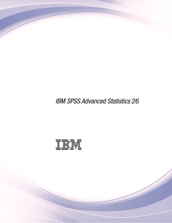
GLM Multivariate Profile PlotsProfile plots (interaction plots) are useful for comparing marginal means in your model. A profile plot isa line plot in which each point indicates the estimated marginal mean of a dependent variable (adjustedfor any covariates) at one level of a factor. The levels of a second factor can be used to make separatelines. Each level in a third factor can be used to create a separate plot. All factors are available for plots.Profile plots are created for each dependent variable.A profile plot of one factor shows whether the estimated marginal means are increasing or decreasingacross levels. For two or more factors, parallel lines indicate that there is no interaction between factors,which means that you can investigate the levels of only one factor. Nonparallel lines indicate aninteraction.Figure 1. Nonparallel plot (left) and parallel plot (right)After a plot is specified by selecting factors for the horizontal axis and, optionally, factors for separatelines and separate plots, the plot must be added to the Plots list.GLM Multivariate Post Hoc ComparisonsPost hoc multiple comparison tests. Once you have determined that differences exist among the means,post hoc range tests and pairwise multiple comparisons can determine which means differ. Comparisonsare made on unadjusted values. The post hoc tests are performed for each dependent variable separately.The Bonferroni and Tukey's honestly significant difference tests are commonly used multiple comparisontests. The Bonferroni test, based on Student's t statistic, adjusts the observed significance level for the factthat multiple comparisons are made. Sidak's t test also adjusts the significance level and provides tighterbounds than the Bonferroni test. Tukey's honestly significant difference test uses the Studentized rangestatistic to make all pairwise comparisons between groups and sets the experimentwise error rate to theerror rate for the collection for all pairwise comparisons. When testing a large number of pairs of means,Tukey's honestly significant difference test is more powerful than the Bonferroni test. For a small numberof pairs, Bonferroni is more powerful.Hochberg's GT2 is similar to Tukey's honestly significant difference test, but the Studentized maximummodulus is used. Usually, Tukey's test is more powerful. Gabriel's pairwise comparisons test also usesthe Studentized maximum modulus and is generally more powerful than Hochberg's GT2 when the cellsizes are unequal. Gabriel's test may become liberal when the cell sizes vary greatly.Dunnett's pairwise multiple comparison t test compares a set of treatments against a single controlmean. The last category is the default control category. Alternatively, you can choose the first category.You can also choose a two-sided or one-sided test. To test that the mean at any level (except the controlcategory) of the factor is not equal to that of the control category, use a two-sided test. To test whetherthe mean at any level of the factor is smaller than that of the control category, select Control. Likewise,to test whether the mean at any level of the factor is larger than that of the control category, select Control.Ryan, Einot, Gabriel, and Welsch (R-E-G-W) developed two multiple step-down range tests. Multiplestep-down procedures first test whether all means are equal. If all means are not equal, subsets of meansAdvanced statistics5

are tested for equality. R-E-G-W F is based on an F test and R-E-G-W Q is based on the Studentizedrange. These tests are more powerful than Duncan's multiple range test and Student-Newman-Keuls(which are also multiple step-down procedures), but they are not recommended for unequal cell sizes.When the variances are unequal, use Tamhane's T2 (conservative pairwise comparisons test based on a ttest), Dunnett's T3 (pairwise comparison test based on the Studentized maximum modulus),Games-Howell pairwise comparison test (sometimes liberal), or Dunnett's C (pairwise comparison testbased on the Studentized range).Duncan's multiple range test, Student-Newman-Keuls (S-N-K), and Tukey's b are range tests that rankgroup means and compute a range value. These tests are not used as frequently as the tests previouslydiscussed.The Waller-Duncan t test uses a Bayesian approach. This range test uses the harmonic mean of thesample size when the sample sizes are unequal.The significance level of the Scheffé test is designed to allow all possible linear combinations of groupmeans to be tested, not just pairwise comparisons available in this feature. The result is that the Scheffétest is often more conservative than other tests, which means that a larger difference between means isrequired for significance.The least significant difference (LSD) pairwise multiple comparison test is equivalent to multipleindividual t tests between all pairs of groups. The disadvantage of this test is that no attempt is made toadjust the observed significance level for multiple comparisons.Tests displayed. Pairwise comparisons are provided for LSD, Sidak, Bonferroni, Games-Howell,Tamhane's T2 and T3, Dunnett's C, and Dunnett's T3. Homogeneous subsets for range tests are providedfor S-N-K, Tukey's b, Duncan, R-E-G-W F, R-E-G-W Q, and Waller. Tukey's honestly significant differencetest, Hochberg's GT2, Gabriel's test, and Scheffé's test are both multiple comparison tests and range tests.GLM Estimated Marginal MeansSelect the factors and interactions for which you want estimates of the population marginal means in thecells. These means are adjusted for the covariates, if any.v Compare main effects. Provides uncorrected pairwise comparisons among estimated marginal meansfor any main effect in the model, for both between- and within-subjects factors. This item is availableonly if main effects are selected under the Display Means For list.v Confidence interval adjustment. Select least significant difference (LSD), Bonferroni, or Sidakadjustment to the confidence intervals and significance. This item is available only if Compare maineffects is selected.Specifying Estimated Marginal Means1. From the menus choose one of the procedures available under Analyze General Linear Model.2. In the main dialog, click EM Means.GLM SaveYou can save values predicted by the model, residuals, and related measures as new variables in the DataEditor. Many of these variables can be used for examining assumptions about the data. To save the valuesfor use in another IBM SPSS Statistics session, you must save the current data file.Predicted Values. The values that the model predicts for each case.vv6Unstandardized. The value the model predicts for the dependent variable.Weighted. Weighted unstandardized predicted values. Available only if a WLS variable was previouslyselected.IBM SPSS Advanced Statistics 26

vStandard error. An estimate of the standard deviation of the average value of the dependent variablefor cases that have the same values of the independent variables.Diagnostics. Measures to identify cases with unusual combinations of values for the independentvariables and cases that may have a large impact on the model.v Cook's distance. A measure of how much the residuals of all cases would change if a particular casewere excluded from the calculation of the regression coefficients. A large Cook's D indicates thatexcluding a case from computation of the regression statistics changes the coefficients substantially.v Leverage values. Uncentered leverage values. The relative influence of each observation on the model'sfit.Residuals. An unstandardized residual is the actual value of the dependent variable minus the valuepredicted by the model. Standardized, Studentized, and deleted residuals are also available. If a WLSvariable was chosen, weighted unstandardized residuals are available.vUnstandardized. The difference between an observed value and the value predicted by the model.vWeighted. Weighted unstandardized residuals. Available only if a WLS variable was previouslyselected.vStandardized. The residual divided by an estimate of its standard deviation. Standardized residuals,which are also known as Pearson residuals, have a mean of 0 and a standard deviation of 1.vStudentized. The residual divided by an estimate of its standard deviation that varies from case to case,depending on the distance of each case's values on the independent variables from the means of theindependent variables.vDeleted. The residual for a case when that case is excluded from the calculation of the regressioncoefficients. It is the difference between the value of the dependent variable and the adjusted predictedvalue.Coefficient Statistics. Writes a variance-covariance matrix of the parameter estimates in the model to anew dataset in the current session or an external IBM SPSS Statistics data file. Also, for each dependentvariable, there will be a row of parameter estimates, a row of standard errors of the parameter estimates,a row of significance values for the t statistics corresponding to the parameter estimates, and a row ofresidual degrees of freedom. For a multivariate model, there are similar rows for each dependentvariable. When Heteroskedasticity-consistent statistics is selected (only available for univariate models),the variance-covariance matrix is calculated using a robust estimator, the row of standard errors displaysthe robust standard errors, and the significance values reflect the robust errors. You can use this matrixfile in other procedures that read matrix files.GLM Multivariate OptionsOptional statistics are available from this dialog box. Statistics are calculated using a fixed-effects model.Display. Select Descriptive statistics to produce observed means, standard deviations, and counts for allof the dependent variables in all cells. Estimates of effect size gives a partial eta-squared value for eacheffect and each parameter estimate. The eta-squared statistic describes the proportion of total variabilityattributable to a factor. Select Observed power to

v Bayesian Statistics analysis makes inference via generating a posterior distribution of the unknown parameters that is based on observed data and a priori information on the parameters. Bayesian Statistics in IBM SPSS Statistics focuses particularly on the inference on the mean of one-sample