Transcription
iIBM SPSS Advanced Statistics 20
Note: Before using this information and the product it supports, read the general informationunder Notices on p. 166.This edition applies to IBM SPSS Statistics 20 and to all subsequent releases and modificationsuntil otherwise indicated in new editions.Adobe product screenshot(s) reprinted with permission from Adobe Systems Incorporated.Microsoft product screenshot(s) reprinted with permission from Microsoft Corporation.Licensed Materials - Property of IBM Copyright IBM Corporation 1989, 2011.U.S. Government Users Restricted Rights - Use, duplication or disclosure restricted by GSA ADPSchedule Contract with IBM Corp.
PrefaceIBM SPSS Statistics is a comprehensive system for analyzing data. The Advanced Statisticsoptional add-on module provides the additional analytic techniques described in this manual. TheAdvanced Statistics add-on module must be used with the SPSS Statistics Core system and iscompletely integrated into that system.About IBM Business AnalyticsIBM Business Analytics software delivers complete, consistent and accurate information thatdecision-makers trust to improve business performance. A comprehensive portfolio of businessintelligence, predictive analytics, financial performance and strategy management, and analyticapplications provides clear, immediate and actionable insights into current performance and theability to predict future outcomes. Combined with rich industry solutions, proven practices andprofessional services, organizations of every size can drive the highest productivity, confidentlyautomate decisions and deliver better results.As part of this portfolio, IBM SPSS Predictive Analytics software helps organizations predictfuture events and proactively act upon that insight to drive better business outcomes. Commercial,government and academic customers worldwide rely on IBM SPSS technology as a competitiveadvantage in attracting, retaining and growing customers, while reducing fraud and mitigatingrisk. By incorporating IBM SPSS software into their daily operations, organizations becomepredictive enterprises – able to direct and automate decisions to meet business goals and achievemeasurable competitive advantage. For further information or to reach a representative visithttp://www.ibm.com/spss.Technical supportTechnical support is available to maintenance customers. Customers may contact TechnicalSupport for assistance in using IBM Corp. products or for installation help for one of thesupported hardware environments. To reach Technical Support, see the IBM Corp. web siteat http://www.ibm.com/support. Be prepared to identify yourself, your organization, and yoursupport agreement when requesting assistance.Technical Support for StudentsIf you’re a student using a student, academic or grad pack version of any IBMSPSS software product, please see our special online Solutions for Education(http://www.ibm.com/spss/rd/students/) pages for students. If you’re a student using auniversity-supplied copy of the IBM SPSS software, please contact the IBM SPSS productcoordinator at your university.Customer ServiceIf you have any questions concerning your shipment or account, contact your local office. Pleasehave your serial number ready for identification. Copyright IBM Corporation 1989, 2011.iii
Training SeminarsIBM Corp. provides both public and onsite training seminars. All seminars feature hands-onworkshops. Seminars will be offered in major cities on a regular basis. For more information onthese seminars, go to g.Additional PublicationsThe SPSS Statistics: Guide to Data Analysis, SPSS Statistics: Statistical Procedures Companion,and SPSS Statistics: Advanced Statistical Procedures Companion, written by Marija Norušis andpublished by Prentice Hall, are available as suggested supplemental material. These publicationscover statistical procedures in the SPSS Statistics Base module, Advanced Statistics moduleand Regression module. Whether you are just getting starting in data analysis or are ready foradvanced applications, these books will help you make best use of the capabilities found withinthe IBM SPSS Statistics offering. For additional information including publication contentsand sample chapters, please see the author’s website: http://www.norusis.comiv
Contents1Introduction to Advanced Statistics12GLM Multivariate Analysis2GLM Multivariate Model . . . . . . . . . . . . . . . . . . . . . . . . . . . . . . . . . . . . . . . . . . . . . . . . . . . . . . . . 4Build Terms . . . . . . . . . . . . . . . . . . . . . . . . . . . . . . . . . . . . . . . . . . . . . . . . . . . . . . . . . . . . . . 4Sum of Squares . . . . . . . . . . . . . . . . . . . . . . . . . . . . . . . . . . . . . . . . . . . . . . . . . . . . . . . . . . . 5GLM Multivariate Contrasts . . . . . . . . . . . . . . . . . . . . . . . . . . . . . . . . . . . . . . . . . . . . . . . . . . . . . 6Contrast Types. . . . . . . . . . . . . . . . . . . . . . . . . . . . . . . . . . . . . . . . . . . . . . . . . . . . . . . . . . . . 6GLM Multivariate Profile Plots . . . . . . . . . . . . . . . . . . . . . . . . . . . . . . . . . . . . . . . . . . . . . . . . . . . 7GLM Multivariate Post Hoc Comparisons . . . . . . . . . . . . . . . . . . . . . . . . . . . . . . . . . . . . . . . . . . . 8GLM Save. . . . . . . . . . . . . . . . . . . . . . . . . . . . . . . . . . . . . . . . . . . . . . . . . . . . . . . . . . . . . . . . . . . 10GLM Multivariate Options . . . . . . . . . . . . . . . . . . . . . . . . . . . . . . . . . . . . . . . . . . . . . . . . . . . . . . . 11GLM Command Additional Features . . . . . . . . . . . . . . . . . . . . . . . . . . . . . . . . . . . . . . . . . . . . . . . 123GLM Repeated Measures14GLM Repeated Measures Define Factors . . . . . . . . . . . . . . . . . . . . . . . . . . . . . . . . . . . . . . . . . . . 17GLM Repeated Measures Model . . . . . . . . . . . . . . . . . . . . . . . . . . . . . . . . . . . . . . . . . . . . . . . . . 18Build Terms . . . . . . . . . . . . . . . . . . . . . . . . . . . . . . . . . . . . . . . . . . . . . . . . . . . . . . . . . . . . . . 19Sum of Squares . . . . . . . . . . . . . . . . . . . . . . . . . . . . . . . . . . . . . . . . . . . . . . . . . . . . . . . . . . . 19GLM Repeated Measures Contrasts . . . . . . . . . . . . . . . . . . . . . . . . . . . . . . . . . . . . . . . . . . . . . . . 20Contrast Types. . . . . . . . . . . . . . . . . . . . . . . . . . . . . . . . . . . . . . . . . . . . . . . . . . . . . . . . . . . . 21GLM Repeated Measures Profile Plots . . . . . . . . . . . . . . . . . . . . . . . . . . . . . . . . . . . . . . . . . . . . . 21GLM Repeated Measures Post Hoc Comparisons . . . . . . . . . . . . . . . . . . . . . . . . . . . . . . . . . . . . . 22GLM Repeated Measures Save. . . . . . . . . . . . . . . . . . . . . . . . . . . . . . . . . . . . . . . . . . . . . . . . . . . 24GLM Repeated Measures Options . . . . . . . . . . . . . . . . . . . . . . . . . . . . . . . . . . . . . . . . . . . . . . . . 25GLM Command Additional Features . . . . . . . . . . . . . . . . . . . . . . . . . . . . . . . . . . . . . . . . . . . . . . . 264Variance Components Analysis28Variance Components Model . . . . . . . . . . . . . . . . . . . . . . . . . . . . . . . . . . . . . . . . . . . . . . . . . . . . 30Build Terms . . . . . . . . . . . . . . . . . . . . . . . . . . . . . . . . . . . . . . . . . . . . . . . . . . . . . . . . . . . . . . 30Variance Components Options . . . . . . . . . . . . . . . . . . . . . . . . . . . . . . . . . . . . . . . . . . . . . . . . . . . 31Sum of Squares (Variance Components) . . . . . . . . . . . . . . . . . . . . . . . . . . . . . . . . . . . . . . . . 32v
Variance Components Save to New File . . . . . . . . . . . . . . . . . . . . . . . . . . . . . . . . . . . . . . . . . . . . 33VARCOMP Command Additional Features . . . . . . . . . . . . . . . . . . . . . . . . . . . . . . . . . . . . . . . . . . . 335Linear Mixed Models34Linear Mixed Models Select Subjects/Repeated Variables . . . . . . . . . . . . . . . . . . . . . . . . . . . . . . 36Linear Mixed Models Fixed Effects . . . . . . . . . . . . . . . . . . . . . . . . . . . . . . . . . . . . . . . . . . . . . . . . 37Build Non-Nested Terms . . . . . . .Build Nested Terms . . . . . . . . . . .Sum of Squares . . . . . . . . . . . . . .Linear Mixed Models Random Effects .37383839Linear Mixed Models Estimation . . . . . . . . . . . . . . . . . . . . . . . . . . . . . . . . . . . . . . . . . . . . . . . . . . 41Linear Mixed Models Statistics. . . . . . . . . . . . . . . . . . . . . . . . . . . . . . . . . . . . . . . . . . . . . . . . . . . 42Linear Mixed Models EM Means . . . . . . . . . . . . . . . . . . . . . . . . . . . . . . . . . . . . . . . . . . . . . . . . . 43Linear Mixed Models Save . . . . . . . . . . . . . . . . . . . . . . . . . . . . . . . . . . . . . . . . . . . . . . . . . . . . . . 44MIXED Command Additional Features. . . . . . . . . . . . . . . . . . . . . . . . . . . . . . . . . . . . . . . . . . . . . . 456Generalized Linear Models46Generalized Linear Models Response . . . . . . . . . . . . . . . . . . . . . . . . . . . . . . . . . . . . . . . . . . . . . . 50Generalized Linear Models Reference Category. . . . . . . . . . . . . . . . . . . . . . . . . . . . . . . . . . . 51Generalized Linear Models Predictors . . . . . . . . . . . . . . . . . . . . . . . . . . . . . . . . . . . . . . . . . . . . . 52Generalized Linear Models Options . . . . . . . . . . . . . . . . . . . . . . . . . . . . . . . . . . . . . . . . . . . . 53Generalized Linear Models Model . . . . . . . . . . . . . . . . . . . . . . . . . . . . . . . . . . . . . . . . . . . . . . . . 54Generalized Linear Models Estimation . . . . . . . . . . . . . . . . . . . . . . . . . . . . . . . . . . . . . . . . . . . . . 56Generalized Linear Models Initial Values . . . . . . . . . . . . . . . . . . . . . . . . . . . . . . . . . . . . . . . . 58Generalized Linear Models Statistics . . . . . . . . . . . . . . . . . . . . . . . . . . . . . . . . . . . . . . . . . . . . . . 59Generalized Linear Models EM Means . . . . . . . . . . . . . . . . . . . . . . . . . . . . . . . . . . . . . . . . . . . . . 61Generalized Linear Models Save. . . . . . . . . . . . . . . . . . . . . . . . . . . . . . . . . . . . . . . . . . . . . . . . . . 63Generalized Linear Models Export . . . . . . . . . . . . . . . . . . . . . . . . . . . . . . . . . . . . . . . . . . . . . . . . 65GENLIN Command Additional Features . . . . . . . . . . . . . . . . . . . . . . . . . . . . . . . . . . . . . . . . . . . . . 667Generalized Estimating Equations68Generalized Estimating Equations Type of Model . . . . . . . . . . . . . . . . . . . . . . . . . . . . . . . . . . . . . 72Generalized Estimating Equations Response . . . . . . . . . . . . . . . . . . . . . . . . . . . . . . . . . . . . . . . . . 75Generalized Estimating Equations Reference Category . . . . . . . . . . . . . . . . . . . . . . . . . . . . . 76vi
Generalized Estimating Equations Predictors . . . . . . . . . . . . . . . . . . . . . . . . . . . . . . . . . . . . . . . . 77Generalized Estimating Equations Options . . . . . . . . . . . . . . . . . . . . . . . . . . . . . . . . . . . . . . . 78Generalized Estimating Equations Model . . . . . . . . . . . . . . . . . . . . . . . . . . . . . . . . . . . . . . . . . . . 79Generalized Estimating Equations Estimation . . . . . . . . . . . . . . . . . . . . . . . . . . . . . . . . . . . . . . . . 81Generalized Estimating Equations Initial Values . . . . . . . . . . . . . . . . . . . . . . . . . . . . . . . . . . . 82Generalized Estimating Equations Statistics . . . . . . . . . . . . . . . . . . . . . . . . . . . . . . . . . . . . . . . . . 84Generalized Estimating Equations EM Means . . . . . . . . . . . . . . . . . . . . . . . . . . . . . . . . . . . . . . . . 86Generalized Estimating Equations Save. . . . . . . . . . . . . . . . . . . . . . . . . . . . . . . . . . . . . . . . . . . . . 88Generalized Estimating Equations Export . . . . . . . . . . . . . . . . . . . . . . . . . . . . . . . . . . . . . . . . . . . 90GENLIN Command Additional Features . . . . . . . . . . . . . . . . . . . . . . . . . . . . . . . . . . . . . . . . . . . . . 918Generalized linear mixed models93Obtaining a generalized linear mixed model . . . . . . . . . . . . . . . . . . . . . . . . . . . . . . . . . . . . . . . . . 95Target . . . . . . . . . . . . . . . . . . . . . . . . . . . . . . . . . . . . . . . . . . . . . . . . . . . . . . . . . . . . . . . . . . . . . 97Fixed Effects . . . . . . . . . . . . . . . . . . . . . . . . . . . . . . . . . . . . . . . . . . . . . . . . . . . . . . . . . . . . . . . 100Add a Custom Term . . . . . . . . . . . . . . . . . . . . . . . . . . . . . . . . . . . . . . . . . . . . . . . . . . . . . . . 101Random Effects . . . . . . . . . . . . . . . . . . . . . . . . . . . . . . . . . . . . . . . . . . . . . . . . . . . . . . . . . . . . . 103Random Effect Block . . . . . . . . . . . . . . . . . . . . . . . . . . . . . . . . . . . . . . . . . . . . . . . . . . . . . . 104Weight and Offset . . . . . . . . . . . . . . . . . . . . . . . . . . . . . . . . . . . . . . . . . . . . . . . . . . . . . . . . . . . 106Build Options . . . . . . . . . . . . . . . . . . . . . . . . . . . . . . . . . . . . . . . . . . . . . . . . . . . . . . . . . . . . . . . 107Estimated Means . . . . . . . . . . . . . . . . . . . . . . . . . . . . . . . . . . . . . . . . . . . . . . . . . . . . . . . . . . . . 108Save . . . . . . . . . . . . . . . . . . . . . . . . . . . . . . . . . . . . . . . . . . . . . . . . . . . . . . . . . . . . . . . . . . . . . 110Model view . . . . . . . . . . . . . . . . . . . . . . . . . . . . . . . . . . . . . . . . . . . . . . . . . . . . . . . . . . . . . . . . 111Model Summary . . . . . . . . . . . . . . . .Data Structure . . . . . . . . . . . . . . . . .Predicted by Observed . . . . . . . . . . .Classification . . . . . . . . . . . . . . . . . .Fixed Effects . . . . . . . . . . . . . . . . . . .Fixed Coefficients . . . . . . . . . . . . . . .Random Effect Covariances . . . . . . .Covariance Parameters . . . . . . . . . .Estimated Means: Significant EffectsEstimated Means: Custom Effects . . .9.Model Selection Loglinear r Analysis Define Range. . . . . . . . . . . . . . . . . . . . . . . . . . . . . . . . . . . . . . . . . . . . . . . . . 125vii
Loglinear Analysis Model . . . . . . . . . . . . . . . . . . . . . . . . . . . . . . . . . . . . . . . . . . . . . . . . . . . . . . 126Build Terms . . . . . . . . . . . . . . . . . . . . . . . . . . . . . . . . . . . . . . . . . . . . . . . . . . . . . . . . . . . . . 126Model Selection Loglinear Analysis Options . . . . . . . . . . . . . . . . . . . . . . . . . . . . . . . . . . . . . . . . 127HILOGLINEAR Command Additional Features . . . . . . . . . . . . . . . . . . . . . . . . . . . . . . . . . . . . . . . 12710 General Loglinear Analysis128General Loglinear Analysis Model . . . . . . . . . . . . . . . . . . . . . . . . . . . . . . . . . . . . . . . . . . . . . . . 130Build Terms . . . . . . . . . . . . . . . . . . . . . . . . . . . . . . . . . . . . . . . . . . . . . . . . . . . . . . . . . . . . . 130General Loglinear Analysis Options. . . . . . . . . . . . . . . . . . . . . . . . . . . . . . . . . . . . . . . . . . . . . . . 131General Loglinear Analysis Save. . . . . . . . . . . . . . . . . . . . . . . . . . . . . . . . . . . . . . . . . . . . . . . . . 132GENLOG Command Additional Features . . . . . . . . . . . . . . . . . . . . . . . . . . . . . . . . . . . . . . . . . . . 13211 Logit Loglinear Analysis133Logit Loglinear Analysis Model . . . . . . . . . . . . . . . . . . . . . . . . . . . . . . . . . . . . . . . . . . . . . . . . . . 135Build Terms . . . . . . . . . . . . . . . . . . . . . . . . . . . . . . . . . . . . . . . . . . . . . . . . . . . . . . . . . . . . . 136Logit Loglinear Analysis Options . . . . . . . . . . . . . . . . . . . . . . . . . . . . . . . . . . . . . . . . . . . . . . . . . 136Logit Loglinear Analysis Save . . . . . . . . . . . . . . . . . . . . . . . . . . . . . . . . . . . . . . . . . . . . . . . . . . . 137GENLOG Command Additional Features . . . . . . . . . . . . . . . . . . . . . . . . . . . . . . . . . . . . . . . . . . . 13712 Life Tables139Life Tables Define Events for Status Variables . . . . . . . . . . . . . . . . . . . . . . . . . . . . . . . . . . . . . . . 141Life Tables Define Range. . . . . . . . . . . . . . . . . . . . . . . . . . . . . . . . . . . . . . . . . . . . . . . . . . . . . . . 141Life Tables Options . . . . . . . . . . . . . . . . . . . . . . . . . . . . . . . . . . . . . . . . . . . . . . . . . . . . . . . . . . . 141SURVIVAL Command Additional Features . . . . . . . . . . . . . . . . . . . . . . . . . . . . . . . . . . . . . . . . . . 14213 Kaplan-Meier Survival Analysis143Kaplan-Meier Define Event for Status Variable . . . . . . . . . . . . . . . . . . . . . . . . . . . . . . . . . . . . . . 144Kaplan-Meier Compare Factor Levels . . . . . . . . . . . . . . . . . . . . . . . . . . . . . . . . . . . . . . . . . . . . . 145Kaplan-Meier Save New Variables . . . . . . . . . . . . . . . . . . . . . . . . . . . . . . . . . . . . . . . . . . . . . . . 146Kaplan-Meier Options. . . . . . . . . . . . . . . . . . . . . . . . . . . . . . . . . . . . . . . . . . . . . . . . . . . . . . . . . 146KM Command Additional Features . . . . . . . . . . . . . . . . . . . . . . . . . . . . . . . . . . . . . . . . . . . . . . . 147viii
14 Cox Regression Analysis148Cox Regression Define Categorical Variables . . . . . . . . . . . . . . . . . . . . . . . . . . . . . . . . . . . . . . . 149Cox Regression Plots . . . . . . . . . . . . . . . . . . . . . . . . . . . . . . . . . . . . . . . . . . . . . . . . . . . . . . . . . 151Cox Regression Save New Variables. . . . . . . . . . . . . . . . . . . . . . . . . . . . . . . . . . . . . . . . . . . . . . 152Cox Regression Options . . . . . . . . . . . . . . . . . . . . . . . . . . . . . . . . . . . . . . . . . . . . . . . . . . . . . . . 153Cox Regression Define Event for Status Variable. . . . . . . . . . . . . . . . . . . . . . . . . . . . . . . . . . . . . 153COXREG Command Additional Features . . . . . . . . . . . . . . . . . . . . . . . . . . . . . . . . . . . . . . . . . . . 15315 Computing Time-Dependent Covariates155Computing a Time-Dependent Covariate . . . . . . . . . . . . . . . . . . . . . . . . . . . . . . . . . . . . . . . . . . . 155Cox Regression with Time-Dependent Covariates Additional Features . . . . . . . . . . . . . . . . . 156AppendicesA Categorical Variable Coding Schemes157Deviation . . . . . . . . . . . . . . . . . . . . . . . . . . . . . . . . . . . . . . . . . . . . . . . . . . . . . . . . . . . . . . . . . . 157Simple . . . . . . . . . . . . . . . . . . . . . . . . . . . . . . . . . . . . . . . . . . . . . . . . . . . . . . . . . . . . . . . . . . . . 158Helmert . . . . . . . . . . . . . . . . . . . . . . . . . . . . . . . . . . . . . . . . . . . . . . . . . . . . . . . . . . . . . . . . . . . 158Difference . . . . . . . . . . . . . . . . . . . . . . . . . . . . . . . . . . . . . . . . . . . . . . . . . . . . . . . . . . . . . . . . . 159Polynomial . . . . . . . . . . . . . . . . . . . . . . . . . . . . . . . . . . . . . . . . . . . . . . . . . . . . . . . . . . . . . . . . . 159Repeated . . . . . . . . . . . . . . . . . . . . . . . . . . . . . . . . . . . . . . . . . . . . . . . . . . . . . . . . . . . . . . . . . . 160Special . . . . . . . . . . . . . . . . . . . . . . . . . . . . . . . . . . . . . . . . . . . . . . . . . . . . . . . . . . . . . . . . . . . . 160Indicator. . . . . . . . . . . . . . . . . . . . . . . . . . . . . . . . . . . . . . . . . . . . . . . . . . . . . . . . . . . . . . . . . . . 161B Covariance Structures162C Notices166Index169ix
ChapterIntroduction to Advanced Statistics1The Advanced Statistics option provides procedures that offer more advanced modeling optionsthan are available through the Statistics Base option. GLM Multivariate extends the general linear model provided by GLM Univariate to allowmultiple dependent variables. A further extension, GLM Repeated Measures, allows repeatedmeasurements of multiple dependent variables. Variance Components Analysis is a specific tool for decomposing the variability in adependent variable into fixed and random components. Linear Mixed Models expands the general linear model so that the data are permitted toexhibit correlated and nonconstant variability. The mixed linear model, therefore, providesthe flexibility of modeling not only the means of the data but the variances and covariances aswell. Generalized Linear Models (GZLM) relaxes the assumption of normality for the error termand requires only that the dependent variable be linearly related to the predictors through atransformation, or link function. Generalized Estimating Equations (GEE) extends GZLMto allow repeated measurements. General Loglinear Analysis allows you to fit models for cross-classified count data, andModel Selection Loglinear Analysis can help you to choose between models. Logit Loglinear Analysis allows you to fit loglinear models for analyzing the relationshipbetween a categorical dependent and one or more categorical predictors. Survival analysis is available through Life Tables for examining the distribution oftime-to-event variables, possibly by levels of a factor variable; Kaplan-Meier SurvivalAnalysis for examining the distribution of time-to-event variables, possibly by levels ofa factor variable or producing separate analyses by levels of a stratification variable; andCox Regression for modeling the time to a specified event, based upon the values of givencovariates. Copyright IBM Corporation 1989, 2011.1
ChapterGLM Multivariate Analysis2The GLM Multivariate procedure provides regression analysis and analysis of variance formultiple dependent variables by one or more factor variables or covariates. The factor variablesdivide the population into groups. Using this general linear model procedure, you can test nullhypotheses about the effects of factor variables on the means of various groupings of a jointdistribution of dependent variables. You can investigate interactions between factors as well asthe effects of individual factors. In addition, the effects of covariates and covariate interactionswith factors can be included. For regression analysis, the independent (predictor) variables arespecified as covariates.Both balanced and unbalanced models can be tested. A design is balanced if each cell inthe model contains the same number of cases. In a multivariate model, the sums of squaresdue to the effects in the model and error sums of squares are in matrix form rather than thescalar form found in univariate analysis. These matrices are called SSCP (sums-of-squares andcross-products) matrices. If more than one dependent variable is specified, the multivariateanalysis of variance using Pillai’s trace, Wilks’ lambda, Hotelling’s trace, and Roy’s largest rootcriterion with approximate F statistic are provided as well as the univariate analysis of variancefor each dependent variable. In addition to testing hypotheses, GLM Multivariate producesestimates of parameters.Commonly used a priori contrasts are available to perform hypothesis testing. Additionally,after an overall F test has shown significance, you can use post hoc tests to evaluate differencesamong specific means. Estimated marginal means give estimates of predicted mean values forthe cells in the model, and profile plots (interaction plots) of these means allow you to visualizesome of the relationships easily. The post hoc multiple comparison tests are performed for eachdependent variable separately.Residuals, predicted values, Cook’s distance, and leverage values can be saved as new variablesin your data file for checking assumptions. Also available are a residual SSCP matrix, which is asquare matrix of sums of squares and cross-products of residuals, a residual covariance matrix,which is the residual SSCP matrix divided by the degrees of freedom of the residuals, and theresidual correlation matrix, which is the standardized form of the residual covariance matrix.WLS Weight allows you to specify a variable used to give observations different weightsfor a weighted least-squares (WLS) analysis, perhaps to compensate for different precision ofmeasurement.Example. A manufacturer of plastics measures three properties of plastic film: tear resistance,gloss, and opacity. Two rates of extrusion and two different amounts of additive are tried, andthe three properties are measured under each combination of extrusion rate and additive amount.The manufacturer finds that the extrusion rate and the amount of additive individually producesignificant results but that the interaction of the two factors is not significant.Methods. Type I, Type II, Type III, and Type IV sums of squares can be used to evaluate differenthypotheses. Type III is the default. Copyright IBM Corporation 1989, 2011.2
3GLM Multivariate AnalysisStatistics. Post hoc range tests and multiple comparisons: least significant difference, Bonferroni,Sidak, Scheffé, Ryan-Einot-Gabriel-Welsch multiple F, Ryan-Einot-Gabriel-Welsch multiplerange, Student-Newman-Keuls, Tukey’s honestly significant difference, Tukey’s b, Duncan,Hochberg’s GT2, Gabriel, Waller Duncan t test, Dunnett (one-sided and two-sided), Tamhane’sT2, Dunnett’s T3, Games-Howell, and Dunnett’s C. Descriptive statistics: observed means,standard deviations, and counts for all of the dependent variables in all cells; the Levene test forhomogeneity of variance; Box’s M test of the homogeneity of the covariance matrices of thedependent variables; and Bartlett’s test of sphericity.Plots. Spread-versus-level, residual, and profile (interaction).Data. The dependent variables should be quantitative. Factors are categorical and can havenumeric values or string values. Covariates are quantitative variables that are related to thedependent variable.Assumptions. For dependent variables, the data are a random sample of vectors from a multivariatenormal population; in the population, the variance-covariance matrices for all cells are thesame. Analysis of variance is robust to departures from normality, although the data should besymmetric. To check assumptions, you can use homogeneity of variances tests (including Box’sM) and spread-versus-level plots. You can also examine residuals and residual plots.Related procedures. Use the Explore procedure to examine the data before doing an analysisof variance. For a single dependent variable, use GLM Univariate. If you measured the samedependent variables on several occasions for each subject, use GLM Repeated Measures.Obtaining GLM Multivariate TablesE From the menus choose:Analyze General Linear Model Multivariate.Figure 2-1Multivariate dialog boxE Select at least two dependent variables.
4Chapter 2Optionally, you can specify Fixed Factor(s), Covariate(s), and WLS Weight.GLM Multivariate ModelFigure 2-2Multivariate Model dialog boxSpecify Model. A full factorial model contains all factor main effects, all covariate main effects,and all factor-by-factor interactions. It does not contain covariate interactions. Select Custom tospecify only a subset of interactions or to specify factor-by-covariate interactions. You mustindicate all of the terms to be included in the model.Factors and Covariates. The factors and covariates are listed.Model. The model depends on the nature of your data. After selecting Custom, you can select themain effects and interactions that are of interest in your analysis.Sum of squares. The method of calculating the sums of squares. For balanced or unbalancedmodels with no missing cells, the Type III sum-of-squares method is most commonly used.Include intercept in model. The intercept is usually included in the model. If you can assume thatthe data pass through the origin, you can exclude the intercept.Build TermsFor the selected factors and covariates:Interaction. Creates the highest-level interaction term of all selected variables. This is the default.Main effects. Creates a main-effects term for each variable selected.All 2-way. Creates all possible two-way interactions of the selected variables.
5GLM Multivariate AnalysisAll 3-way. Creates all possible three-way interactions of the selected variables.All 4-way. Creates all possible four-way interactions of the selected variables.All 5-way. Creates all possible five-way interactions of the selected variables.Sum of SquaresFor the model, you can choose a type of sums of squares. Type III is the most commonly usedand is the default.Type I. This method is also known as the hierarchical decomposition of the sum-of-squaresmethod. Each term is adjusted for only the term that precedes it in the model. Type I sums ofsquares are commonly used for: A balanced ANOVA model in which any main effects are specified before any first-orderinteraction effects, any first-order interaction effects are specified before any second-orderinteraction effects, and so on. A polynomial regression model in which any lower-order terms
IBM SPSS Statistics is a comprehensive system for analyzing data. The Advanced Statistics optional add-on module provides the additional analytic techniques described in this manual. The Advanced Statistics add-on module must be used with the SPSS Statistics Core system and is completely integrated into that system. About IBM Business Analytics