WIXLIB

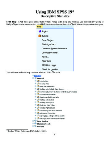
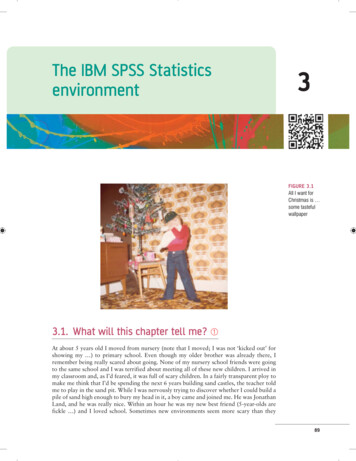
CHAPTE R 3 TH E I B M SPSS STATI STI CS E NV I R O N M E N Tplace). You can also useto select various preferences such as the font that isused for the output. The default preferences are fine for most purposes. This menu deals with system specifications such as whether you have grid lineson the data editor, or whether you display value labels (exactly what value labels arewill become clear later). This menu allows you to make changes to the data editor. The important featuresare, which is used to insert a new variable into the data editor (i.e., adda column);, which is used to add a new row of data between two existingrows of data;, which is used to split the file by a grouping variable (see Section5.3.2.4); and, which is used to run analyses on only a selected sample ofcases. You should use this menu if you want to manipulate one of your variables insome way. For example, you can use recode to change the values of certain variables(e.g., if you wanted to adopt a slightly different coding scheme for some reason) – seeSPSS Tip 10.2. The compute function is also useful for transforming data (e.g., youcan create a new variable that is the average of two existing variables). This functionallows you to carry out any number of calculations on your variables (see Section5.4.4.2). The fun begins here, because the statistical procedures lurk in this menu.Below is a brief guide to the options in the statistics menu that will be used during thecourse of this book (this is only a small portion of what is available):{This menu is for conducting descriptive statistics (mean,mode, median, etc.), frequencies and general data exploration. There is also acommand called crosstabs that is useful for exploring frequency data and performing tests such as chi-square, Fisher’s exact test and Cohen’s kappa.{This is where you can find t-tests (related and unrelated –Chapter 9) and one-way independent ANOVA (Chapter 11).{This menu is for more complex ANOVA such as two-way(unrelated, related or mixed), one-way ANOVA with repeated measures and multivariate analysis of variance (MANOVA) – see Chapters 12 to 16.{This menu can be used for running multilevel linear models(MLMs). At the time of writing I know absolutely nothing about these, but seeingas I’ve promised to write a chapter on them I’d better go and do some reading.With luck you’ll find a chapter on it later in the book, or 30 blank sheets of paper.It could go either way.{It doesn’t take a genius to work out that this is where thecorrelation techniques are kept. You can do bivariate correlations such as Pearson’sR, Spearman’s rho (U) and Kendall’s tau (W ) as well as partial correlations (seeChapter 6).{There are a variety of regression techniques available inSPSS. You can do simple linear regression, multiple linear regression (Chapter 8)and more advanced analyses such as logistic regression (Chapter 19).{Loglinear analysis is hiding in this menu, waiting for you,and ready to pounce like a tarantula from its burrow (Chapter 18).{You’ll find factor analysis here (Chapter 17).{Here you’ll find reliability analysis (Chapter 17).93

D I S C O VE R I N G STAT I ST I C S US I N G I BM S P SS STAT I ST I C S94{There are a variety of non-parametric statistics availablesuch the chi-square goodness-of-fit statistic, the binomial test, the Mann–Whitneytest, the Kruskal–Wallis test, Wilcoxon’s test and Friedman’s ANOVA (Chapter 6). SPSS has some graphing facilities and this menu is used to access the ChartBuilder (see Chapter 4). The types of graphs you can do include bar charts, histograms, scatterplots, box–whisker plots, pie charts and error bar graphs. In this menu there is an option,, that allows you to comment on your data set. This can be quite useful because you can write yourself notesabout from where the data come, or the date they were collected and so on. SPSS sell several add-ons that can be accessed through this menu. For example, they have a program called Sample Power that computes the sample size requiredfor studies, and power statistics (see Section 2.6.1.7). However, because most peoplewon’t have these add-ons (including me) I’m not going to discuss them in the book. This menu allows you to switch from window to window. So, if you’re looking at the output and you wish to switch back to your data sheet, you can do so usingthis menu. There are icons to shortcut most of the options in this menu, so it isn’tparticularly useful. This is an invaluable menu because it offers you online help on both the systemitself and the statistical tests. The statistics help files are fairly incomprehensible attimes (the program is not designed to teach you statistics) and are certainly no substitute for acquiring a good book like this, erm, I mean acquiring a good knowledge ofyour own. However, they can get you out of a sticky situation.At the top of the data editor window are a set of icons (see Figure 3.3) that are shortcutsto frequently used facilities in the menus. Using the icons saves you time. Below is a brieflist of these icons and their functions.This icon gives you the option to open a previously saved file (if you are in thedata editor, SPSS assumes you want to open a data file; if you are in the outputviewer, it will offer to open a viewer file).This icon allows you to save files. It will save the file you are currently workingon (be it data or output). If the file hasn’t already been saved it will produce theSave Data As dialog box.S PSS T I P 3 . 1Save time and avoid RSI By default, when you try to open a file from SPSS it will go to the directory in which the program is stored on yourcomputer. This is fine if you happen to store all of your data and output in that folder, but if not then you will findyourself spending time navigating around your computer trying to find your data. If you use SPSS as much asI do then this has two consequences: (1) all those seconds have added up to weeks navigating my computerwhen I could have been doing something useful like playing my drum kit; (2) I have increased my chances ofgetting RSI in my wrists, and if I’m going to get RSI in my wrists I can think of more enjoyable ways to achieveit than navigating my computer (drumming again, obviously). Luckily, we can avoid wrist death by telling SPSSwhere we’d like it to start looking for files. Selectto open the Options dialog box below and selectthe File Locations tab.

CHAPTE R 3 TH E I B M SPSS STATI STI CS E NV I R O N M E N T95 This dialog box allows you to select a folder in which SPSS will initially look for data files and other files. Forexample, I keep all of my data files in a single folder called, rather unimaginatively, ‘Data’. In the dialog box hereI have clicked onand then navigated to my data folder. SPSS will use this as the default location when I tryto open files and my wrists are spared the indignity of RSI. You can also select the option for SPSS to use theLast folder used, in which case SPSS remembers where you were last time it was loaded and uses that folderwhen you open files.This icon activates a dialog box for printing whatever you are currently workingon (either the data editor or the output). The exact print options will depend onthe printer you use. By default SPSS will print everything in the output window,so a useful way to save trees is to print only a selection of the output (see SPSSTip 3.5).Clicking on this icon will activate a list of the last 12 dialog boxes that you used.You can select any box from the list and it will appear on the screen. This iconmakes it easy for you to repeat parts of an analysis.This icon implies to me (what with the big arrow and everything) that if youclick on it SPSS will send a miniaturizing ray out of your monitor that shrinksyou and then sucks you into a red cell in the data editor, where you will spendthe rest of your days fighting decimal points with your bare hands. Fortunately,this icon does not do this, but instead enables you to go directly to a case (a rowin the data editor). This button is useful if you are working on large data files: ifyou were analysing a survey with 3000 respondents it would get pretty tediousscrolling down the data sheet to find the responses of participant 2407. Byclicking on this icon you can skip straight to the case by typing the case numberrequired (in our example 2407) into this dialog box:

96D I S C O VE R I N G STAT I ST I C S US I N G I BM S P SS STAT I ST I C S Similar to the previous icon, clicking this button activates a function that enablesyou to go directly to a variable (i.e., a column in the data editor). As before, thisis useful when working with big data files in which you have many columns ofdata. In the example below, we have a data file with 23 variables and each variable represents a question on a questionnaire and is named accordingly (we’ll usethis data file, SAQ.sav, in Chapter 17). We can use this icon to activate the Go Todialog box, but this time to find a variable. Notice that a drop-down box lists thefirst 10 variables in the data editor, but you can scroll down to go to others. Clicking on this icon opens a dialog box that shows you the variables in the dataeditor and summary information about each one. The dialog box below showsthe information for the file that we used for the previous icon. We have selectedthe first variable in this file, and we can see the variable name (question 01), thelabel (Statistics makes me cry), the measurement level (ordinal), and the valuelabels (e.g., the number 1 represents the response of ‘strongly agree’).

CHAPTE R 3 TH E I B M SPSS STATI STI CS E NV I R O N M E N T97I initially thought that this icon would allow me to spy on my neighbours,but this shining diamond of excitement was snatched cruelly from me by thecloaked thief that is SPSS. Instead, click this button to search for words ornumbers in your data file and output window. In the data editor it will searchwithin the variable (column) that is currently active. This option is useful if,for example, you realize from a graph of your data that you have typed 20.02instead of 2.02 (see Section 4.4): you can simply search for 20.02 within thatvariable and replace that value with 2.02: Clicking on this icon inserts a new case in the data editor (so it creates a blankrow at the point that is currently highlighted in the data editor). This function isvery useful if you need to add new data at a particular point in the data editor.Clicking on this icon creates a new variable to the left of the variable that is currentlyactive (to activate a variable simply click once on the name at the top of the column).Clicking on this icon is a shortcut to thefunction (see Section5.3.2.4). There are often situations in which you might want to analyse groups ofcases separately. In SPSS we differentiate groups of cases by using a coding variable(see Section 3.5.2.3), and this function lets us divide our output by such a variable.For example, we might test males and females on their statistical ability. We cancode each participant with a number that represents their gender (e.g., 1 female,0 male). If we then want to know the mean statistical ability of each gender wesimply ask the computer to split the file by the variable Gender. Any subsequentanalyses will be performed on the men and women separately. There are situationsacross many disciplines where this might be useful: sociologists and economistsmight want to look at data from different geographic locations separately, biologists might wish to analyse different groups of mutated mice, and so on.This icon shortcuts to thefunction. This function is necessarywhen we come to input frequency data (see Section 18.5.2.2) and is useful forsome advanced issues in survey sampling.This icon is a shortcut to thefunction. If you want to analyseonly a portion of your data, this is the option for you. This function allows youto specify what cases you want to include in the analysis.Clicking on this icon will either display or hide the value labels of any coding variables. We often group people together and use a coding variable to letthe computer know that a certain participant belongs to a certain group. Forexample, if we coded gender as 1 female, 0 male then the computer knowsthat every time it comes across the value 1 in the Gender column, that person isa female. If you press this icon, the coding will appear on the data editor ratherthan the numerical values; so, you will see the words male and female in theGender column rather than a series of numbers. This idea will become clear inSection 3.5.2.3.

D I S C O VE R I N G STAT I ST I C S US I N G I BM S P SS STAT I ST I C S983.5.1. Entering data into the data editor When you first load SPSS it will provide a blank data editor with the title Untitled1 (thisof course is daft because once it has been given the title ‘untitled’ it ceases to be untitled).When inputting a new set of data, you must input your data in a logical way. The SPSS dataeditor is arranged such that each row represents data from one entity while each columnrepresents a variable. There is no discrimination between independent and dependent variables: both types should be placed in a separate column. The key point is that each rowrepresents one entity’s data (be that entity a human, mouse, tulip, business, or water sample). Therefore, any information about that case should be entered across the data editor.For example, imagine you were interested in sex differences in perceptions of pain createdby hot and cold stimuli. You could place some people’s hands in a bucket of very cold waterfor a minute and ask them to rate how painful they thought the experience was on a scaleof 1 to 10. You could then ask them to hold a hot potato and again measure their perception of pain. Imagine I was a participant. You would have a single row representing mydata, so there would be a different column for my name, my gender, my pain perceptionfor cold water and my pain perception for a hot potato: Andy, male, 7, 10.The column with the information about my gender is a grouping variable: I can belongto either the group of males or the group of females, but not both. As such, this variable isa between-group variable (different people belong to different groups). Rather than representing groups with words, in SPSS we use numbers. This involves assigning each group anumber, and then telling SPSS which number represents which group. Therefore, betweengroup variables are represented by a single column in which the group to which the personbelonged is defined using a number (see Section 3.5.2.3). For example, we might decidethat if a person is male then we give them the number 0, and if they’re female we give themthe number 1. We then tell SPSS that every time it sees a 1 in a particular column the personis a female, and every time it sees a 0 the person is a male. Variables that specify to which ofseveral groups a person belongs can be used to split data files (so in the pain example youcould run an analysis on the male and female participants separately – see Section 5.3.2.4).Finally, the two measures of pain are a repeated measure (all participants were subjectedto hot and cold stimuli). Therefore, levels of this variable (see SPSS Tip 3.2) can be enteredin separate columns (one for pain to a hot stimulus and one for pain to a cold stimulus).S PSS T I P 3 . 2Entering data There is a simple rule for how variables should be placed in the SPSS data editor: data from different thingsgo in different rows of the data editor, whereas data from the same things go in different columns of the dataeditor. As such, each person (or mollusc, goat, organization, or whatever you have measured) is representedin a different row. Data within each person (or mollusc, etc.) go in different columns. So, if you’ve prodded yourmollusc, or human, several times with a pencil and measured how much it twitches as an outcome, then eachprod will be represented by a column.In experimental research this means that any variable measured with the same participants (a repeated measure) should be represented by several columns (each column representing one level of the repeated-measuresvariable). However, any variable that defines different groups of things (such as when a between-groups designis used and different participants are assigned to different levels of the independent variable) is defined usinga single column. This idea will become clearer as you learn about how to carry out specific procedures. (Thisgolden rule is broken in mixed models, but until Chapter 19 we can overlook this annoying anomaly.)

CHAPTE R 3 TH E I B M SPSS STATI STI CS E NV I R O N M E N T99The data editor is made up of lots of cells, which are boxes in which data values can beplaced. When a cell is active it becomes highlighted in orange (as in Figure 3.3). You canmove around the data editor, from cell to cell, using the arrow keys m n p o (found onthe right of the keyboard) or by clicking the mouse on the cell that you wish to activate.To enter a number into the data editor simply move to the cell in which you want to placethe data value, type the value, then press the appropriate arrow button for the direction inwhich you wish to move. So, to enter a row of data, move to the far left of the row, typethe value and then press o (this process inputs the value and then moves you into the nextcell on the right).The first step in entering your data is to create some variables using the variable view ofthe data editor, and then to input your data using the data view of the data editor. We’ll gothrough these two steps by working through an example.3.5.2. The variable view Before we input any data into the data editor, we need to create the variables. To create variables we use the variable view of the data editor. To access this view click on the‘Variable View’ tab at the bottom of the data editor (); the contents of thewindow will change (see Figure 3.4).FIGURE 3.4The ‘VariableView’ of theSPSS DataEditor Every row of the variable view represents a variable, and you set characteristics of a particular variable by entering information into the following labelled columns (play aroundand you’ll get the hang of it):You can enter a name in this column for each variable. This name willappear at the top of the corresponding column in the data view, andhelps you to identify variables in the data view. You can more or lesswrite what you like, but there are certain symbols you can’t use (mainlysymbols that have other uses in SPSS such as , , &), and you can’t usespaces. (It can be useful to use a ‘hard space’, which replaces the spacewith an underscore; for example, Andy Field instead of Andy Field.) Ifyou use a character that SPSS doesn’t like you’ll get an error messagesaying that the variable name is invalid when you click on a differentcell, or try to move off the cell using the arrow keys.You can have different types of data. Mostly you will use numeric variables (which means that the variable contains numbers and is the default).You will come across string variables, which consist of strings of letters. If you wanted to type in people’s names, for example, you would

100D I S C O VE R I N G STAT I ST I C S US I N G I BM S P SS STAT I ST I C Sneed to change the variable type to be string rather than numeric. Youcan also have currency variables (i.e., s, s, s) and date variables (e.g.,21-06-1973)By default, when a new variable is created, SPSS sets it up to be numericand to store 8 digits/characters, but you can change this value by typinga new number in this column in the dialog box. For numeric variables8 digits is fine (unless you have very large numbers), but for string variables you will often make this value bigger (you can’t write a lot in only8 characters). This characteristic differs fromin that it affectswhat is stored in the variable rather than what is displayed in the dataeditor.Another default setting is to have 2 decimal places displayed. (You’llnotice that if you don’t change this option then when you type in wholenumbers to the data editor SPSS adds a decimal place with two zerosafter it, which can be disconcerting.) If you want to change the numberof decimal places for a given variable then replace the 2 with a new valueor increase or decrease the value using .The name of the variable (see above) has some restrictions on characters, and you also wouldn’t want to use huge long names at the top ofyour columns (they become hard to read). Therefore, you can write alonger variable description in this column. This may seem pointless, butis actually one of the best habits you can get into (see SPSS Tip 3.3).This column is for assigning numbers to represent group

3.2. Versions of IBM SPSS Statistics This book is based primarily on version 21 of IBM SPSS Statistics; however, don’t be fooled too much by version numbers because SPSS release ‘new’ versions each year, and as you might imagine, not much changes in a year. Occasionally IBM h