Transcription
NUMERICAL SIMULATION OF THE TATARA BRIDGE AND ITS AERODYNAMICSTABILITY OPTIMIZATIONbySen WangB.S. Engineering, China University of Geoscience (Beijing), 2013Submitted to the Graduate Faculty ofThe Swanson School of Engineering in partial fulfillmentof the requirements for the degree ofMaster of Science in Civil EngineeringUniversity of Pittsburgh2015
UNIVERSITY OF PITTSBURGHSWANSON SCHOOL OF ENGINEERINGThis thesis was presentedbySen WangIt was defended onMarch 27, 2015and approved byJeen-Shang Lin, ScD, Associate Professor,Department of Civil and Environmental EngineeringThesis Co-advisor: John Brigham, PhD, Assistant Professor,Department of Civil and Environmental EngineeringThesis Advisor: Qiang Yu, PhD, Assistant Professor,Department of Civil and Environmental Engineeringii
Copyright by Sen Wang2015iii
NUMERICAL SIMULATION OF THE TATARA BRIDGE AND ITSAERODYNAMIC STABILITY OPTIMIZATIONSen Wang, M.S.University of Pittsburgh, 2015The importance of bridge aerodynamic stability was immediately realized after the catastrophicfailure of the Tacoma Narrows Bridge in 1940. Since then aerodynamic control system that usingmoveable flaps to increase the aerodynamic stability of bridge has been attracting increasinginterests and become an important aspect in bridge aerodynamic designs. In last two decades, asignificant growth in bridge span and structural complexity has been witnessed. This means thataerodynamic control system is an indispensable part for modern large-span bridge, and the activecontrol system appears as a promising solution to improve the aerodynamic stability when bridgemain span exceeds 3000 m. The purpose of this thesis is to study the effect of activeaerodynamic control system with two sharp shape control devices installed on the edges ofbridge decks by FEM simulation. Here, the Tatara Bridge is analyzed via FEM softwareABAQUS and SOLIDWORKS. This study consists of FEM modal analysis of the bridge, windtunnel test simulation and wind effect test modeling for the entire bridge under wind blowingfrom inclined directions. In the bridge modal analysis, the first 400 vibration mode shapes andtheir corresponding frequencies are calculated through Lanczos method solver in ABAQUS andthe first order mode shape is found to be lateral bending of the deck. Therefore, the target is tooptimize the deck shape to reduce the lateral aerodynamic force. To achieve this goal, 9 deckshapes are designed and tested under wind load from 15 different directions in the wind tunneltest simulation through SOLIDWORKS. The result of this test shows the optimized deck shapesiv
can significantly reduce the lateral aerodynamic force. Then the wind effect tests of the entirebridge before and after optimization are performed and compared in ABAQUS. As shown in theresults, the displacement of midspan is decreased, especially in lateral direction. The results ofthis study indicate that this actively transformable sharp control surface can significantly reducethe response of the bridge under lateral aerodynamic force.v
TABLE OF CONTENTSACKNOWLEDGEMENTS .XV1.0INTRODUCTION . 11.1BACKGROUND . 11.2LITERATURE REVIEW . 61.2.1Modal analysis. 61.2.2Wind tunnel test and CFD simulation . 81.2.3Aerodynamic optimization. 111.32.0STUDY PLAN . 14FEM MODAL ANALYSIS OF THE TATARA BRIDGE. 162.1BASIC INFORMATION OF THE TATARA BRIDGE . 162.2THE THEORY USED IN SIMULATION OF THE TATARA BRIDGE. 232.2.1Finite element method . 232.2.2Theory of modal analysis . 252.2.2.1 Analysis of free vibration frequencies . 262.2.2.2 Analysis of free vibration mode shapes . 272.3BRIDGE MODELING . 292.4RESULT AND DISCUSSION OF MODAL ANALYSIS . 342.5CONCLUSION OF MODAL ANALYSIS . 38vi
3.0WIND TUNNEL TEST BY CFD SIMULATION . 403.1DESCRIPTION OF MODIFIED DECK SHAPES . 413.2HORIZONTAL WIND TEST SIMULATION . 433.2.1Horizontal wind test simulation . 433.2.2Result and conclusion of horizontal wind test in SOLIDWORKS . 483.2.2.1 Result of horizontal wind tunnel test simulation. 503.2.2.2 Conclusion of horizontal wind tunnel test simulation . 563.3NON-HORIZONTAL WIND TUNNEL TEST SIMULATION . 573.3.1Description of selected deck shapes . 573.3.2Non-horizontal wind tunnel test modeling . 583.3.3Result and conclusion of non-horizontal wind test . 613.3.3.1 Result of non-horizontal wind test . 613.3.3.2 Conclusion. 684.0OPTIMIZATION . 694.1DESCRIPTION OF OPTIMIZATION . 694.2OPTIMIZATION PROCESS . 714.3RESULT OF OPTIMIZATION . 734.4CONCLUSION . 795.0SUMMARY AND RECOMMENDATIONS OF FUTURE WORKS . 805.1SUMMARY . 805.2RECOMMENDATIONS . 81APPENDIX A . 82APPENDIX B . 90vii
BIBLIOGRAPHY . 93viii
LIST OF TABLESTable 2.1 Section properties of cables . 21Table 2.2 First 30 frequencies and corresponding vibration shape description . 38Table 3.1 Test results of Deck1 and Deck2 . 51Table 3.2 Test results of Group 1. 51Table 3.3 Comparison from Deck 1 to Deck 7 . 51Table 3.4 Test results of Group 2. 54Table 3.5 Comparison between Deck 1, Deck 2 and Deck in Group 2 . 54Table 3.6 Decomposition of wind velocity according to different wind attacked angle. . 59Table 3.7 Minimum magnitude of horizontal force with different angle . 66Table 3.8 Comparison of minimum horizontal force of each deck shape . 67Table 4.1 Best optimized deck shape choice with different wind attacked angles . 72Table 5.1 Records of original deck (Deck 1) . 83Table 5.2 Records of Deck 3. 84Table 5.3 Records of Deck4. 85Table 5.4 Records of Deck 6. 86Table 5.5 Midspan displacement before optimization . 87Table 5.6 Midspan displacement after optimization . 88ix
Table 5.7 Midspan displacement increasing after optimization . 89x
LIST OF FIGURESFigure 1.1 Ancient stone bridge . 2Figure 1.2 The Akashi Kaikyō Bridge . 2Figure 1.3 The Russky Bridge . 3Figure 1.4 Active aerodynamic control system of bridge by Larsen (1992) . 5Figure 1.5 The half of solid model by Ishak (2006) . 9Figure 1.6 Comparison of CFD and experimental test by Ishak (2006) . 10Figure 1.7 DNW-NWB wind tunnel (Ciobaca et al 2006) . 11Figure 1.8 AWB wind tunnel (Ciobaca et al 2006) . 11Figure 1.9 Active control methods by Ostenfeld and Larsen (1992) . 13Figure 1.10 Active control methods by Hansen and Palle (1998) . 13Figure 2.1 Nishi-Seto Expressway (Authority 1999) . 17Figure 2.2 Location of the Tatara Bridge on the map (Authority 1999). 17Figure 2.3 General dimensions of the Tatara Bridge (Yabuno 2003). 18Figure 2.4 Cross-section of girders (main girder section) (unit: mm) (Yabuno 2003) . 19Figure 2.5 General dimension of main tower (Yabuno 2003) . 20Figure 2.6 Section profile of main tower (Authority 1999) . 22Figure 2.7 Indent of cable surface (Yabuno 2003) . 22xi
Figure 2.8 Process of finite element method . 24Figure 2.9 Example of mesh . 25Figure 2.10 Global coordinate system of the bridge model . 30Figure 2.11 8-node brick element . 31Figure 2.12 Cable coupled with girder . 31Figure 2.13 Boundary condition at bottom of main tower. 33Figure 2.14 Boundary condition at side span. 34Figure 2.15 Distribution of first 400 frequencies. 34Figure 2.16 First vibration mode . 35Figure 2.17 Second vibration mode . 35Figure 2.18 Third vibration mode . 36Figure 2.19 Fourth vibration mode . 36Figure 2.20 Fifth vibration mode . 36Figure 2.21 15th vibration mode . 37Figure 2.22 20th vibration mode . 37Figure 2.23 30th vibration mode . 37Figure 3.1 Deck shape of original deck (Deck 1) . 42Figure 3.2 Optimized deck shapes of Group 1 (Deck 2 to 7) . 42Figure 3.3 Optimized deck shapes of Group 2 (Deck 8 to 10) . 43Figure 3.4 Turbulent viscosity of block . 44Figure 3.5 Aerodynamic test of block by SOLIDWORKS FLOW SIMULATION . 44Figure 3.6 Sketch of original deck (Deck 1) . 45Figure 3.7 Solid deck shape of original deck extruded depending on its sketch . 45xii
Figure 3.8 Material properties of air . 46Figure 3.9 Define initial condition . 47Figure 3.10 Computation domain of air region . 47Figure 3.11 Basic mesh control . 48Figure 3.12 Turbulent viscosity of Deck 1 under horizontal wind . 49Figure 3.13 Turbulent viscosity of Deck 4 under horizontal wind . 49Figure 3.14 Normalized aerodynamic forces vs. the vertical of sharp tip . 52Figure 3.15 Aerodynamic forces comparison between Deck 1 and decks in Group1 . 52Figure 3.16 Normalized aerodynamic forces vs. the extended horizontal distance of sharp tip . 53Figure 3.17 Aerodynamic forces comparison between Deck 1 and decks in Group2 . 55Figure 3.18 Deck shape selected for wind tunnel test simulation of non-horizontal wind. 58Figure 3.19 Deck 4 solid model in SOLIDWORKS . 59Figure 3.20 Deck in horizontal air flow . 60Figure 3.21 Deck in non-horizontal air flow . 60Figure 3.22 Definition of positive wind attacked angle . 61Figure 3.23 Horizontal force vs. wind attacking angle . 63Figure 3.24 Vertical force vs. wind attacking angle . 63Figure 3.25 Total force vs. wind attacking angle. 64Figure 3.26 Moment vs. wind attacking angle . 64Figure 3.27 Drag coefficient vs. wind attacking angle . 65Figure 3.28 Lifting coefficient vs. wind attacking angle . 65Figure 3.29 Moment coefficient vs. wind attacking angle. 66Figure 3.30 Deck moving direction sketch . 67xiii
Figure 4.1 Wind speed amplitude vs. time . 70Figure 4.2 Maximum lateral displacement vs. wind attacked angle . 74Figure 4.3 Increasing of max lateral displacement vs. wind attacked angle. 74Figure 4.4 Lateral vibration range vs. wind attacked angle . 75Figure 4.5 Increasing of lateral vibration range vs. wind attacked angle . 75Figure 4.6 Maximum vertical displacement vs. wind attacking angle . 76Figure 4.7 Increasing of vertical vibration range vs. wind attacking angle . 77Figure 4.8 Vertical vibration range vs. wind attacking angle . 77Figure 4.9 Vertical vibration range vs. wind attacking angle . 78Figure 4.10 Displacement at 0 degree wind attacked angle (U2: lateral, U3: vertical) . 79Figure 5.1 Displacement of Deck1 at 0 degree . 90Figure 5.2 Displacement of optimized deck at 0 degree . 91Figure 5.3 Displacement of Deck1 at 2 degree . 91Figure 5.4 Displacement of optimized deck at 3 degree . 92Figure 5.5 Displacement of optimized deck at 4 degree . 92xiv
ACKNOWLEDGEMENTSFirst, I would like to express my sincerest gratitude to my advisor Dr. Yu and co-advisor Dr.John Brigham for providing me the opportunity to do the research and supporting me throughoutmy graduate studies with their patience and knowledge. I could not finish my thesis without theirguidance and encouragement.I would also like to acknowledge my committee member, Dr. Jeen-Shang Lin. Thankyou for your precious time and insightful advice.Many thanks to Teng Tong, the PhD student of Dr. Yu. Thank you for helping me buildthe model, guiding me while I was performing the analysis and giving me suggestions.Furthermore, I would like to extend my appreciation to Chunlin Pan, the PhD student ofDr. Yu, for helping me understanding numerical simulation and mechanical analysis.Finally, I would like to take this opportunity to express my thanks to my parents forgiving birth to me and their continuous support throughout my life.xv
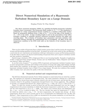
1.01.1INTRODUCTIONBACKGROUND“Bridge” is a word that generally stands for a structure helping people cross rivers for more thanone thousand years. In ancient time, the bridges, as shown in Figure 1.1 (Wikipedia 2014), weremade of wood and stone, which limited the length of main span. And it is also the reason whythere were so many multi-arch bridges in ancient time. At that time, the only load was inducedby pedestrians and as a result, the bridge design in ancient time was based on static mechanicalanalysis. However, nowadays, the advanced mechanics and material science enables us to buildbridges of stupendous size, both for main span and total length, which has been well witnessed inrecent 2 decades. The Akashi Kaikyō Bridge built in 1998, for instance, has so far the longestmain span (1991 m) in suspension bridges all over the world, as shown in Figure 1.2 (Wikipedia2015). The Russky Bridge, as shown in Figure 1.3 (Wikipedia 2015), which was finished 3 yearsago in Russia as the longest cable-stayed bridge in the world has a 1104 m long main span. Andother 3 of the 4 longest cable-stayed bridges whose main spans are around 1000 m long werefinished subsequently in 2008, 2009 and 2010 in China. The overall longest bridge on earth, theDanyang–Kunshan Grand Bridge, with a total length of 164,800 m completed in 2010 in China(Wikipedia 2015), shows that bridges can also be built over the sea now. As demonstrated by1
these amazing bridges, the developing speed of bridges is beyond imagination and the difficultiesin designing and construction process are much more challenging than any old bridges.Figure 1.1 Ancient stone bridgeFigure 1.2 The Akashi Kaikyō Bridge2
Figure 1.3 The Russky BridgeFor larger bridge size, the wind effect on the bridge becomes more obvious, especially inthe high speed wind area where there are many typhoons. There have been many failures ofbridges caused by aerodynamic instability, like the Tacoma Narrows Bridge which collapsed in1940 (Billah et al 1991). Since that time, the aerodynamic analysis has become one of theindispensable mechanical analyses in designing process of bridge.In aerodynamic analysis, determining the natural frequencies of bridge is a veryimportant part. The first recorded bridge failure because of lacking consideration of the naturalfrequencies of the bridge can be traced back to 1831. On April 12th, 1831, the orderly marchingsteps of 74 British soldiers caused the collapse of the Broughton Suspension Bridge. In thiscatastrophe, the frequency of orderly marching steps coincidently matched the natural frequencyof the bridge and led to the resonance of the bridge, which finally caused the collapse of thebridge. Based on this fail experience, the importance of load frequencies and natural frequencies3
of structures was realized by the bridge engineers. This kind of resonance can be induced byother resources, for example, seismic load and wind load. As for the super long bridge, the windload is a critical loading type. Thus, the relation between frequencies of wind loading and naturalfrequencies of structure is important to the stability of bridge. To determine the naturalfrequencies of structures, the modal analysis which is measuring and analyzing the dynamicresponse of structures during excitations is an effective method and became a primary part indesign of bridge.To improve the aerodynamic performance of bridges, the primary target is to lower theresponse to wind as much as possible. In general, there are two types of measures to achieve thisgoal, namely passive aerodynamic measures and active aerodynamic measures. As well known,the real wind is always changing in directions. Unfortunately, the wind tunnel test can onlytheoretically simulate the response of a bridge to the wind from one constant direction, and thismight fail the bridge aerodynamic stability design under non-constant wind. To overcome thisobstacle, a concept comes up using moveable surfaces to reduce wind force by selecting bettershapes under different wind conditions, and based on which these two aforementioned measuresare developed. The passive aerodynamic measures reduce aerodynamic force by improving theconfiguration of cross-section of bridge deck (Xu 2013). For instance, “Slotted deck shape”, adeck with open slots in longitudinal direction of deck, improves the aerodynamic stability andprevents shedding of large vortices. The active aerodynamic measures reduce aerodynamic forceby using actively controlled surfaces, as shown in Figure 1.4 (Xu 2013). The main differencebetween these two is that active control system needs external energy to change the shape whilethe passive control one does not. In fact, aerodynamic shaping and passive measures are notenough to guarantee the aerodynamic stability for a super long bridge that has a main span over4
3000 m. Therefore, the only solution for such a large bridge is to build an active aerodynamiccontrol system that can match all the requirement of any wind attacking angle, such that it canactively change shapes according to the wind conditions, which gives a good guide ofaerodynamic optimization of bridge.However, currently, the practical application of active aerodynamic control system israre. Although it has been an attractive research topic and a lot of researches are focused on it,the tests of the optimization effect on a real bridge with active aerodynamic control system hasnot be accomplished yet. It is reasonable in that engineers want to know the effect of such anexpensive system before it is being built on a real bridge. Therefore, to carry out the test viaFEM modeling in computer as an alternative approach with satisfactorily accurate results, isworthy to try and explore.Figure 1.4 Active aerodynamic control system of bridge by Larsen (1992)In this thesis, the Tatara Bridge was selected as a case study. The main purpose of thisthesis is to explore a new active aerodynamic control design which can reduce the aerodynamicforce at different wind attacking angles by changing deck shapes in theoretical field, and5
therefore enrich the theory of active aerodynamic control system. Additionally, this study willalso try to summarize the relationship between the aerodynamic force of different deck shapesand wind attacking angles. In general, this study includes modal analysis leading to the lowestorder vibration mode of the bridge and its corresponding frequency, and a series of wind tunneltest simulations designed to find the aerodynamic force of different deck cross-section shapesunder different wind conditions. The theoretical background, process, results and relateddiscussions will be introduced in later chapters following a brief literature review about this topic.1.2LITERATURE REVIEW1.2.1 Modal analysisThe modern modal analysis can be traced back in 1960s. At that time, the experimental test is theonly method of modal analysis. This situation has been changed with the invention of somepowerful numerical tools, such as finite element method. Later both the experimental andtheoretical modal analysis has gained large development with the four innovations in late 1970s,namely manufactures of digital signal analyzers, extremely powerful desktop computers,Structural Measurement Systems of San Jose and “FESDEC” the first commercially availablefinite element analysis program (Ramsey 1983). These achievements provide the users an accessto a full complement of experimental and theoretical analysis tools. Examples of the applicationof both approaches on bridges are listed below.In 1994, a research about modal analysis of an arch bridge was published by Deger et al(1994). In this research, a servohyraulic vibration generator was used to excite the bridge and the6
three-axial acceleration measurement devices were placed on 144 points of the bridge in threedimensions to measure the response of the bridge. Meanwhile, a finite element model whichconsisted of 300 CQUAD4 quadrilateral plate elements was built to roughly estimate a feweigen-frequencies of the bridge. The comparison of the results between real experiment and finiteelement model showed that the finite element models were able to reproduce the measuredfrequencies and vibration shapes with satisfactory accuracy.In the same year, a research about modal analysis of a highway bridge was presented byDeger et al (1995). The method used in this research is same as the method mentioned before,involving both experimental and finite element approaches. In this experimental test, the resultswere measured at 94 points in three directions of a bridge. In finite element analysis, the modelconsisted of 1000 CQUAD4 quadrilateral plate elements and 29 CBEAM beam elements. Thecomparison showed that such a finite element model consisted of approximately 1000 elementswas able to capture the eigen-frequencies and corresponding mode shapes.Later, Clemente et al. (1998) published a research about experimental modal analysis ofthe Garigliano cable-stayed bridge. In this research, authors gained the preliminary idea ofdynamic response of the bridge and the selection of optimum sensor locations through the initialtheoretical analysis via finite element model. After the experimental test was finished, theyupgraded the finite element model and used this new model to analyze the vibration of thebridge. Some good matches of the results from both approaches were found. For instance, as forthe first order mode, the experimental frequency was 0.9 and FEM frequency was 0.87. For thesecond order mode, the experimental frequency was 1.30 and FEM frequency was 1.33. Andsimilar results were shown in other modes. Thus, the authors concluded that the numerical model7
was also useful in structural analyses under service loads. Some similar results were found bysome other researchers later (Cunha et al 2001 and Ren 2004).In 2012, Wang et al (2012) published a research about comparative study on buffetingperformance of Suton Bridge. Based on design and
ABAQUS and SOLIDWORKS. This study consists of FEM modal analysis of the bridge, wind tunnel test simulation and wind effect test modeling for the entire bridge under wind blowing from inclined directions. In the bridge modal analysis, the first 400 vibration mode shapes and