Transcription
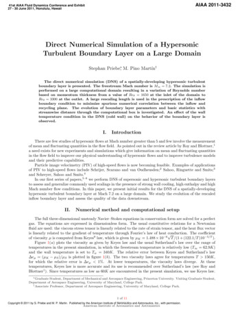
AIAA 2011-343241st AIAA Fluid Dynamics Conference and Exhibit27 - 30 June 2011, Honolulu, HawaiiDirect Numerical Simulation of a HypersonicTurbulent Boundary Layer on a Large DomainStephan Priebe , M. Pino Martı́n†The direct numerical simulation (DNS) of a spatially-developing hypersonic turbulentboundary layer is presented. The freestream Mach number is M 7.2. The simulation isperformed on a large computational domain resulting in a variation of Reynolds numberbased on momentum thickness from a value of Reθ 1650 at the inlet of the domain toReθ 3300 at the outlet. A large rescaling length is used in the prescription of the inflowboundary condition to minimize spurious numerical correlation between the inflow andrecycling plane. The evolution of boundary layer parameters and basic statistics withstreamwise distance through the computational box is investigated. An effect of the walltemperature condition in the DNS (cold wall) on the behavior of the boundary layer isobserved.I.IntroductionThere are few studies of hypersonic flows at Mach number greater than 5 and few involve the measurementof mean and fluctuating quantities in the flow field. As pointed out in the review article by Roy and Blottner,1a need exists for new experiments and simulations which give information on mean and fluctuating quantitiesin the flow field to improve our physical understanding of hypersonic flows and to improve turbulence modelsand their predictive capabilities.Particle image velocimetry (PIV) of high-speed flows is now becoming feasible. Examples of applicationsof PIV to high-speed flows include Schrijer, Scarano and van Oudheusden;2 Sahoo, Ringuette and Smits;3and Schreyer, Sahoo and Smits.4In our first series of papers,5–8 we perform DNS of supersonic and hypersonic turbulent boundary layersto assess and generalize commonly used scalings in the presence of strong wall cooling, high enthalpy and highMach number flow conditions. In this paper, we present initial results for the DNS of a spatially-developinghypersonic turbulent boundary layer at Mach 7.2 on a large domain. We study the evolution of the rescaledinflow boundary layer and assess the quality of the data downstream.II.Numerical method and computational setupThe full three-dimensional unsteady Navier–Stokes equations in conservation form are solved for a perfectgas. The equations are expressed in dimensionless form. The usual constitutive relations for a Newtonianfluid are used: the viscous stress tensor is linearly related to the rate of strain tensor, and the heat flux vectoris linearly related to the gradient of temperature through Fourier’s law of heat conduction. The coefficientof viscosity µ is computed from Keyes9 law, which is given by µK 1.488 10 6 T /(1 (122.1/T )10 5/T ).Figure 1(a) plots the viscosity as given by Keyes law and the usual Sutherland’s law over the range oftemperatures in the present simulation, in which the freestream temperature is relatively low (T 62.9K)and the wall temperature is set to Tw 340K. The relative error between Keyes and Sutherland’s law eµ (µK µS )/µS is plotted in figure 1(b). The two viscosity laws agree for temperatures T 150K,for which the relative error is eµ 1%. At lower temperatures, the viscosity laws diverge. At thesetemperatures, Keyes law is more accurate and its use is recommended over Sutherland’s law (see Roy andBlottner1 ). Since temperatures as low as 60K are encountered in the present simulation, we use Keyes law. Graduate Student, Department of Mechanical and Aerospace Engineering, Princeton University. Visiting Graduate Student,Department of Aerospace Engineering, University of Maryland, College Park.† Associate Professor, Department of Aerospace Engineering, University of Maryland, College Park.1 of 11Copyright 2011 by S. Priebe and M. P. Martin. Published by the American Institute of Aeronautics and Astronautics, Inc., with permission.American Institute of Aeronautics and Astronautics
The governing equations are solved using a fourth-order weighted essentially non-oscillatory (WENO)scheme to discretize the inviscid fluxes. Compared with the original finite-difference WENO scheme introduced by Jiang and Shu,10 which is too dissipative for the accurate computation of compressible flows, thepresent scheme is modified: the modification concerns the linear part of the scheme, that is, the schemein smooth flow regions where a set of optimal WENO weights is engaged. The modification consists inadding a fully-downwinded candidate stencil, which gives a symmetric collection of candidate stencils, andin optimizing the WENO weights to maximize bandwidth-resolving efficiency.11 The resulting symmetricbandwidth-optimized WENO scheme has been extensively validated for the computation of compressibleturbulence and high-speed turbulent boundary layer flows (see Martı́n et al,11 Martı́n,5 and Duan et al6 ).For the discretization of the viscous fluxes, standard fourth-order central differences are used, and timeintegration is performed by means of a third-order low-storage Runge–Kutta method.12The streamwise, spanwise and wall normal coordinates are denoted by x, y and z, respectively. Thecomputational box for the DNS measures Lx /δref 27.0 in the streamwise direction, Ly /δref 10.0 inthe spanwise direction, and Lz /δref 14.2 in the wall normal direction, where δref 5mm is the referencelength which is approximately equal to the boundary layer thickness at the outlet of the computationaldomain (see § III below). The grid has Nx Ny Nz 840 768 150 points (total of approx. 96.8 millionpoints). The grid is uniformly spaced in the streamwise and spanwise directions, whereas it is stretchedin the wall normal direction following a geometric stretching function. The grid resolution at the inlet ofthe computational domain is: x 7.5; y 3.0; the first grid point away from the wall is locatedat z2 0.3, there are 24 points within z 10, and the grid spacing at the edge of the boundary layeris z/δ99 0.04. A grid resolution study has been performed by running temporal DNSs at the sameflow conditions as the present simulation and with several grid resolutions. The results are found to begrid-converged at the resolution used in the present simulation.The freestream conditions in the present DNS are as follows: the velocity is U 1146.1m/s, the densityis ρ 7.43 10 2 kgm 3 , the temperature is T 62.9K, and the Mach number is M 7.21.Concerning the boundary conditions for the simulation, a no-slip isothermal boundary condition is usedat the wall, where the temperature is set to Tw 340K. Supersonic exit boundary conditions are usedat the top and outlet boundaries. Given the high Mach number of the flow and the resulting proximityof the sonic line to the wall, no significant spurious effects are expected to travel from the outlet backinto the domain. Consequently, it is not required to prescribe a sponge layer at the outlet of the domain.Periodicity is prescribed in the spanwise direction. The inflow boundary condition is prescribed by means ofthe recycling-rescaling technique developed by Xu and Martı́n.13 To minimize spurious numerical correlationsand coupling between the inflow plane and the recycling plane, a large rescaling length is required. In thepresent simulation, the recycling plane is located at xrec /δref 26.0 downstream of the inflow plane.III.III.A.ResultsGeneral flow structureThe general flow structure is shown in figures 2 and 3. Figure 2 shows two typical numerical Schlierenvisualizations. Turbulent eddies of length scale O(δ) are visible in the outer region of the boundary layer.Large values of the numerical Schlieren index and hence of magnitude of density gradient are present at theinterface between the irrotational freestream flow and the rotational boundary layer flow. In this high Machnumber flow, the freestream just above the boundary layer contains disturbances that appear to be radiatedfrom the boundary layer structures into the freestream. The visualizations also show the substantial growthof the boundary layer through the computational domain. It may be estimated visually that the boundarylayer thickness approximately doubles from the inlet to the outlet of the domain.Similar observations as from the numerical Schlieren visualizations can be made from figure 3, whichshows the instantaneous three-dimensional structure of the flow. The isosurface of magnitude of densitygradient shown reveals the structure of the bulges of length scale O(δ) in the outer region of the boundarylayer. These structures grow substantially through the computational domain in the streamwise, spanwiseand wall normal direction. The numerical Schlieren visualizations shown on the (x, z)-plane correspondingto the y Ly -boundary of the domain shows the radiation of disturbances from the boundary layer intothe freestream. The disturbances are confined to the vicinity of the boundary layer. At the outlet of thecomputational domain, the disturbances appear to be confined to roughly z/δref 4.2 of 11American Institute of Aeronautics and Astronautics
III.B.Boundary layer parameters and statisticsIn this section, we analyze the evolution with streamwise distance of various boundary layer parameters andbasic statistics. This analysis also serves to investigate the effect of the rescaling inflow boundary conditionon the flow, and to assess what initial portion of the box is unphysical due to the rescaling and must bediscarded.Figure 4(a) shows the evolution of δ99 with streamwise distance, where δ99 is the thickness based on99% of U . The boundary layer grows substantially through the computational domain: at the inlet, thethickness is δ99 /δref 0.45 (δ99 2.25mm); at the outlet, the thickness is approximately δ99 /δref 0.9(δ99 4.5mm).The growth of the boundary layer is also apparent from the evolution of the momentum thickness θ(shown in figure 4(b)) and from the evolution of the displacement thickness δ (shown in figure 4(c)). Atthe outlet, the momentum thickness is approximately θ/δref 0.035 (θ 0.175mm) and the displacementthickness is approximately δ /δref 0.5 (δ 2.5mm).Figure 4(d ) shows the evolution of the shape factor H δ /θ. This quantity is not yet fully converged,but the following behavior appears to develop: the values of H observed near the outlet and inlet of thecomputational domain are approximately equal at H 14. Downstream from the inlet, the value of H dropsdue to the lower local Reynolds number. Downstream of approximately x/δref 5, the shape factor is seento increase gradually with downstream distance as the Reynolds number of the flow increases. Based on theseobservations, it would appear that the first 5 10δref of the computational box are probably unphysical dueto the rescaling and must be discarded, but better converged data is necessary to draw such a conclusionwith confidence.As can be seen from figure 5, the Reynolds number based on momentum thickness Reθ U θ/ν approximately doubles through the computational box, from a value of Reθ 1650 at the inlet to a valueof Reθ 3300 at the outlet.Figure 6(a) shows the evolution of the skin friction coefficient Cf with streamwise distance. The vanDriest II prediction is shown for comparison (see van Driest14 and also Hopkins and Inouye15 ). The relativeerror between the VDII prediction and the DNS results is plotted in figure 6(b). At the inlet of the domain,the value of Cf is approximately 5% above the VDII prediction. With streamwise distance, the value ofCf falls below the VDII prediction and then recovers to pass above it again. Starting at approximatelyx/δref 13, the value of Cf follows the trend of the prediction but is shifted to slightly larger values withan error that is approximately constant at a value of 5%. We attribute this shift to the wall-temperaturecondition in the DNS. The wall temperature is set to Tw 340K, and the adiabatic recovery temperature is2Tr T (1 r(γ 1)/2M ) 645K assuming a recovery factor of r 0.89. The ratio of wall temperatureto adiabatic recovery temperature is thus Tw /Tr 0.53. Duan et al.6 have performed DNS studies toinvestigate the effect of varying wall temperature condition on the properties of super- and hypersonicboundary layers to assess the validity of commonly used scalings. Varying the wall temperature condition ina Mach 5 boundary layer, they find that the skin friction coefficient is generally well predicted by the VDIIscaling across the range of wall temperature conditions. However, there are some slight departures from theprediction, and at the condition with Tw /Tr 0.5, the value of Cf in their simulation lies approximately 5%above the VDII prediction. This is consistent with the departure from the VDII prediction observed in thepresent simulation, and we thus argue that this departure is a wall-temperature effect. In addition, we mayconclude from figure 6 that the boundary layer, which is driven out of equilibrium by the rescaling procedure,recovers to an equilibrium state within approximately x/δref 13 from the inlet. The initial portion of thebox (x/δref 13) is unphysical and must be discarded for the purpose of collecting flow statistics.Figure 7 shows the van Driest transformed velocity u V D at different streamwise locations in the secondhalf of the box. To obtain better statistical convergence, the profiles have been obtained over a streamwisewindow that measures x/δref 2 and is centered at the stations given on the plot. The profiles show a short log law region where u V D (logz )/κ C.The usual value of κ 0.41 fits the data but the additive constant is greater than the usual value ofC 5.2; a value of C 5.9 fits the data. The slight increase in the additive constant C from a value of5.2 to 5.9 is also a wall temperature effect. Duan et al.6 observe this effect in DNS at Mach 5 with varyingwall temperature condition (see figure 5 in their paper). Furthermore, we have performed a grid convergencestudy which shows that the present data are grid converged and that for much finer grids this shift of thelog law to C 5.9 is present unchanged.3 of 11American Institute of Aeronautics and Astronautics
III.C.SpectraIn this section, we present spectra of pressure, streamwise velocity and streamwise mass flux which wereobtained at the recycling station (xrec /δref 26) near the outlet of the domain.Figure 8 shows the spectrum of wall pressure at the recycling station. The energy is broadband andcentered approximately around the characteristic frequency of the boundary layer at f δref /U 1 witha spectral peak at slightly higher frequency of approximately f δref /U 2. There is no energy near thecharacteristic frequency of the rescaling.Figure 9 shows the streamwise velocity and mass flux spectra at three different wall normal locations:(a) the location of the inner peak z 15; (b) the middle of the log layer z 50; and (c) the outer regionz/δref 0.5. There is little difference between the u and ρu-spectra, other than that the latter appear to beshifted to slightly higher frequencies. All spectra are broadband, and the broadband bump shifts to lowerfrequencies as the wall is approached due to the reduction in local convection speed through the boundarylayer. The spectra show that some small energy is still present at the rescaling frequency and at lowerfrequencies. It is possible that these frequencies could be forced by the rescaling. The present data appearsto indicate that such a forcing effect is probably weak, but longer time histories and better resolved spectraare required to fully assess this question.IV.ConclusionsWe have presented initial results for the DNS of a spatially-developing hypersonic turbulent boundarylayer at Mach 7.2 and Reθ 1650 3300. A long computational box is used with a large rescaling length tominimize spurious numerical correlation between the inflow and recycling plane. A significant initial portionof the computational box is affected by the recovery of the boundary layer from the rescaling and must bediscarded. In the second part of the box, relatively good agreement with the VDII prediction is observed andthe van Driest transformed velocity profile follows the log law but with a slightly different additive constant.The slight discrepancies are attributed to the wall temperature condition in the DNS.AcknowledgmentsThis work was supported by the Air Force Office of Scientific Research under grant number AF 9550-091-0464.References1 Roy, C. J. and Blottner, F. G., “Review and assessment of turbulence models for hypersonic flows,” Progress in AerospaceSciences, Vol. 42, 2006.2 Schrijer, F. F. J., Scarano, F., and van Oudheusden, B. W., “Application of PIV in a Mach 7 double-ramp flow,”Experiments in Fluids, Vol. 41, No. 2, 2006, pp. 353–363.3 Sahoo, D., Ringuette, M. J., and Smits, A. J., “Experimental investigation of a hypersonic turbulent boundary layer,”AIAA, 2009, paper 2009-780.4 Schreyer, A.-M., Sahoo, D., and Smits, A. J., “Experimental investigations of a hypersonic shock turbulent boundarylayer interaction,” AIAA, 2011, paper 2011-481.5 Martı́n, M., “Direct numerical simulation of hypersonic turbulent boundary layers. Part 1. Initialization and comparisonwith experiments,” Journal of Fluid Mechanics, Vol. 570, 2007, pp. 347–364.6 Duan, L., Beekman, I., and Martı́n, M. P., “Direct numerical simulation of hypersonic turbulent boundary layers. Part2. Effect of wall temperature,” Journal of Fluid Mechanics, Vol. 655, 2010, pp. 419–445.7 Duan, L., Beekman, I., and Martı́n, M. P., “Direct Numerical Simulation of Hypersonic Turbulent Boundary Layers. PartIII: Effect of Mach Number,” Journal of Fluid Mechanics, Vol. 672, 2011, pp. 245–267.8 Duan, L. and Martı́n, M. P., “Direct Numerical Simulation of Hypersonic Turbulent Boundary Layers. Part IV: Effect ofHigh Enthalpy,” Journal of Fluid Mechanics, 2011, accepted for publication.9 Keyes, F. G., “A summary of viscosity and heat-conduction data for He, A, H , O , N , CO, CO , H O, and air,”22222Transactions of the American Society of Mechanical Engineers, Vol. 73, No. 7, 1951, pp. 589–596.10 Jiang, G.-S. and Shu, C.-W., “Efficient implementation of weighted ENO schemes,” Journal of Computational Physics,Vol. 126, No. 1, 1996, pp. 202–228.11 Martı́n, M., Taylor, E., Wu, M., and Weirs, V., “A bandwidth-optimized WENO scheme for the effective direct numericalsimulation of compressible turbulence,” Journal of Computational Physics, Vol. 220, No. 1, 2006, pp. 270–289.12 Williamson, J. H., “Low-storage Runge–Kutta schemes,” Journal of Computational Physics, Vol. 35, No. 1, 1980, pp. 48– 56.4 of 11American Institute of Aeronautics and Astronautics
13 Xu, S. and Martı́n, M., “Assessment of inflow boundary conditions for compressible turbulent boundary layers,” Physicsof Fluids, Vol. 16, No. 7, 2004, pp. 2623–2639.14 van Driest, E. R., “The problem of aerodynamic heating,” Aeronautical Engineering Review , Vol. 15, No. 10, 1956,pp. 26–41.15 Hopkins, E. J. and Inouye, M., “An evaluation of theories for predicting turbulent skin friction and heat transfer on flatplates at supersonic and hypersonic Mach numbers,” AIAA Journal, Vol. 9, No. 6, 1971, pp. 993–1003.5 of 11American Institute of Aeronautics and Astronautics
SutherlandKeyes2E-0515µ[Pa s] eµ 100150T[K]200250300350400T[K]Figure 1. Comparison of Sutherland’s and Keyes viscosity model for the range of temperatures present in the DNS.6 of 11American Institute of Aeronautics and Astronautics
Figure 2. Typical instantaneous flow visualizations (uncorrelated). Gray-scale contour map of exp( 0.25 ρ ) (numericalSchlieren).7 of 11American Institute of Aeronautics and Astronautics
Figure 3. Typical instantaneous flow visualizations (uncorrelated). Isosurface of magnitude of density gradient ρ δref /ρ 3.0 colored by the wall normal coordinate z. The color map goes from blue (corresponding to thewall) to white (corresponding to z/δref 1). A gray-scale contour map of exp( 0.5 ρ ) is shown on the (x, z)-plane atthe y Ly -boundary of the domain.8 of 11American Institute of Aeronautics and Astronautics
ef15x/δrefFigure 4. Evolution of boundary layer parameters δ99 , θ, δ and H with streamwise Figure 5. Evolution of Reynolds number based on momentum thickness Reθ with streamwise distance.9 of 11American Institute of Aeronautics and Astronautics
1.5DNSvan Driest II51.4Cf 103 eCf x/δrefFigure 6. Evolution of skin friction coefficient Cf and of eCf (Cf,V DII Cf )/Cf with streamwise distance.20u VD1510x/δref 14.0x/δref 18.0x/δref 22.0x/δref 26.0z (1/0.41)logz 5.2 (1/0.41)logz 5.95100101z102 103at different streamwise locations.Figure 7. van Driest transformed velocity u VD1.410-610-710-810-91.20.8E p/prmsfresc22fE δref/U 100fδref/U Figure 8. Spectrum of wall pressure at the recycling location xrec /δref 26.0.10 of 11American Institute of Aeronautics and Astronautics101
11ρuρ1/2uu0.8fresc0.62fE ( )/( )rms0.62fE ( )/( )rms0.8ρu1/2ρ U 100101fδref/U 1ρu1/2ρ uu0.62fE ( )/( )rms0.8fresc0.40.2010-210-1100101fδref/U Figure 9. Spectra at the recycling location xrec /δref 26.0 and at three wall normal locations: z 15, z 50 andz/δref 0.5.11 of 11American Institute of Aeronautics and Astronautics
Stephan Priebe , M. Pino Mart ın † The direct numerical simulation (DNS) of a spatially-developing hypersonic turbulent boundary layer is presented. The freestream Mach number is M 7.2. The simulation is performed on a large computational domain resulting in a variation of Reynolds number