Transcription
Features include:which are based on exciting new areas such as bioengineering.and differential equations.students using this text will be able to apply their new skills to their chosen field.Electronic Textbook Optionsan online resource where students can purchase the complete text in a digital format at almosthalf the cost of the traditional textbook. Students can access the text online for one year.learning, which include full text search, notes and highlighting, and email tools for sharingcontact your salesrepresentative or visit www.CourseSmart.com.Sixth EditionNumericalMethodsfor EngineersChapraCanaleSteven C. ChapraRaymond P. CanaleMD DALIM #1009815 03/12/09 CYAN MAG YELO BLKFor more information, please visit www.mhhe.com/chaprafor Engineersadaptive quadrature.SixthEditionNumerical MethodsThe sixth edition of Numerical Methods for Engineers offers an innovative and accessiblepresentation of numerical methods; the book has earned the Meriam-Wiley award, which isgiven by the American Society for Engineering Education for the best textbook. Because software packages are now regularly used for numerical analysis, this eagerly anticipated revisionmaintains its strong focus on appropriate use of computational tools.
cha01064 fm.qxd3/25/0910:51 AMPage iNumerical Methodsfor EngineersSIXTH EDITIONSteven C. ChapraBerger Chair in Computing and EngineeringTufts UniversityRaymond P. CanaleProfessor Emeritus of Civil EngineeringUniversity of Michigan
cha01064 fm.qxd3/25/0910:51 AMPage iiNUMERICAL METHODS FOR ENGINEERS, SIXTH EDITIONPublished by McGraw-Hill, a business unit of The McGraw-Hill Companies, Inc., 1221 Avenue of the Americas, New York, NY 10020.Copyright 2010 by The McGraw-Hill Companies, Inc. All rights reserved. Previous editions 2006, 2002, and 1998. No part of thispublication may be reproduced or distributed in any form or by any means, or stored in a database or retrieval system, without the priorwritten consent of The McGraw-Hill Companies, Inc., including, but not limited to, in any network or other electronic storage ortransmission, or broadcast for distance learning.Some ancillaries, including electronic and print components, may not be available to customers outside the United States.This book is printed on acid-free paper.1 2 3 4 5 6 7 8 9 0 VNH/VNH 0 9ISBN 978–0–07–340106–5MHID 0–07–340106–4Global Publisher: Raghothaman SrinivasanSponsoring Editor: Debra B. HashDirector of Development: Kristine TibbettsDevelopmental Editor: Lorraine K. BuczekSenior Marketing Manager: Curt ReynoldsProject Manager: Joyce WattersLead Production Supervisor: Sandy LudovissyAssociate Design Coordinator: Brenda A. RolwesCover Designer: Studio Montage, St. Louis, Missouri(USE) Cover Image: BrandX/JupiterImagesCompositor: Macmillan Publishing SolutionsTypeface: 10/12 Times RomanPrinter: R. R. Donnelley Jefferson City, MOAll credits appearing on page or at the end of the book are considered to be an extension of the copyright page.MATLAB is a registered trademark of The MathWorks, Inc.Library of Congress Cataloging-in-Publication DataChapra, Steven C.Numerical methods for engineers / Steven C. Chapra, Raymond P. Canale. — 6th ed.p. cm.Includes bibliographical references and index.ISBN 978–0–07–340106–5 — ISBN 0–07–340106–4 (hard copy : alk. paper)1. Engineering mathematics—Data processing. 2. Numerical calculations—Data processing 3. Microcomputers—Programming. I. Canale, Raymond P. II. Title.TA345.C47 2010518.02462—dc222008054296www.mhhe.com
cha01064 p08.qxd3/25/091:33 PMPage 843PARTIAL DIFFERENTIALEQUATIONSPT8.1MOTIVATIONGiven a function u that depends on both x and y, the partial derivative of u with respect tox at an arbitrary point (x, y) is defined asu(x "x, y) u(x, y) u lim"x 0 x"x(PT8.1)Similarly, the partial derivative with respect to y is defined asu(x, y "y) u(x, y) u lim"y 0 y"y(PT8.2)An equation involving partial derivatives of an unknown function of two or more independent variables is called a partial differential equation, or PDE. For example, 2u 2u 2xy u 1 x2 y2 3u 2u x 2 8u 5y2 x y y! 2 "3 u 3u 6 x x2 x y 2 2u u xu x2 x y(PT8.3)(PT8.4)(PT8.5)(PT8.6)The order of a PDE is that of the highest-order partial derivative appearing in the equation.For example, Eqs. (PT8.3) and (PT8.4) are second- and third-order, respectively.A partial differential equation is said to be linear if it is linear in the unknown functionand all its derivatives, with coefficients depending only on the independent variables. Forexample, Eqs. (PT8.3) and (PT8.4) are linear, whereas Eqs. (PT8.5) and (PT8.6) are not.Because of their widespread application in engineering, our treatment of PDEs willfocus on linear, second-order equations. For two independent variables, such equations canbe expressed in the following general form:A 2u 2u 2u B C 2 D 02 x x y y(PT8.7)where A, B, and C are functions of x and y and D is a function of x, y, u, u/ x , and u/ y.Depending on the values of the coefficients of the second-derivative terms—A, B, C—843
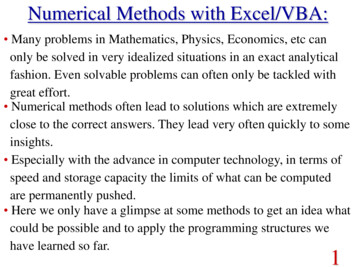
cha01064 p08.qxd8443/25/091:33 PMPage 844PARTIAL DIFFERENTIAL EQUATIONSTABLE PT8.1 Categories into which linear, second-order partial differential equations intwo variables can be classified.B2 ! 4AC 0CategoryExampleEllipticLaplace equation (steady state with two spatial dimensions) 2T 2T! !2 0 x 2 y 0ParabolicHeat conduction equation (time variable with one spatialdimension) T 2T! k ′ !2 t x 0HyperbolicWave equation (time variable with one spatial dimension) 2y1 2y!2 !2 ! xc t 2Eq. (PT8.7) can be classified into one of three categories (Table PT8.1). This classification,which is based on the method of characteristics (for example, see Vichnevetsky, 1981, orLapidus and Pinder, 1981), is useful because each category relates to specific and distinctengineering problem contexts that demand special solution techniques. It should be notedthat for cases where A, B, and C depend on x and y, the equation may actually fall into a different category, depending on the location in the domain for which the equation holds. Forsimplicity, we will limit the present discussion to PDEs that remain exclusively in one ofthe categories.PT8.1.1 PDEs and Engineering PracticeEach of the categories of partial differential equations in Table PT8.1 conforms to specifickinds of engineering problems. The initial sections of the following chapters will be devoted to deriving each type of equation for a particular engineering problem context. Forthe time being, we will discuss their general properties and applications and show how theycan be employed in different physical contexts.Elliptic equations are typically used to characterize steady-state systems. As in theLaplace equation in Table PT8.1, this is indicated by the absence of a time derivative.Thus, these equations are typically employed to determine the steady-state distribution ofan unknown in two spatial dimensions.A simple example is the heated plate in Fig. PT8.1a. For this case, the boundaries ofthe plate are held at different temperatures. Because heat flows from regions of high to lowtemperature, the boundary conditions set up a potential that leads to heat flow from the hotto the cool boundaries. If sufficient time elapses, such a system will eventually reach thestable or steady-state distribution of temperature depicted in Fig. PT8.1a. The Laplaceequation, along with appropriate boundary conditions, provides a means to determine thisdistribution. By analogy, the same approach can be employed to tackle other problems involving potentials, such as seepage of water under a dam (Fig. PT8.1b) or the distributionof an electric field (Fig. PT8.1c).
cha01064 p08.qxd3/25/091:33 PMPage 845845PT8.1 MOTIVATIONHotDamHotCoolFlow lineoructdnCoEquipotentiallineCoolImpermeable rock(a)(b)(c)FIGURE PT8.1Three steady-state distribution problems that can be characterized by elliptic PDEs. (a) Temperature distribution on a heated plate, (b) seepage of water under a dam, and (c) the electricfield near the point of a conductor.HotFIGURE PT8.2(a) A long, thin rod that isinsulated everywhere but at itsend. The dynamics of the onedimensional distribution oftemperature along the rod’slength can be described by aparabolic PDE. (b) The solution,consisting of distributionscorresponding to the state of therod at various times.Cool(a)Tt 3" t(b)t 2t " "ttt 0xIn contrast to the elliptic category, parabolic equations determine how an unknownvaries in both space and time. This is manifested by the presence of both spatial andtemporal derivatives in the heat conduction equation from Table PT8.1. Such cases arereferred to as propagation problems because the solution “propagates,’’ or changes, intime.A simple example is a long, thin rod that is insulated everywhere except at its end(Fig. PT8.2a). The insulation is employed to avoid complications due to heat loss along the
cha01064 p08.qxd3/25/091:33 PM846Page 846PARTIAL DIFFERENTIAL EQUATIONSFIGURE PT8.3A taut string vibrating at a lowamplitude is a simple physicalsystem that can be characterized by a hyperbolic PDE.rod’s length. As was the case for the heated plate in Fig. PT8.1a, the ends of the rod are setat fixed temperatures. However, in contrast to Fig. PT8.1a, the rod’s thinness allows us toassume that heat is distributed evenly over its cross section—that is, laterally. Consequently,lateral heat flow is not an issue, and the problem reduces to studying the conduction of heatalong the rod’s longitudinal axis. Rather than focusing on the steady-state distribution intwo spatial dimensions, the problem shifts to determining how the one-dimensional spatialdistribution changes as a function of time (Fig. PT8.2b). Thus, the solution consists of aseries of spatial distributions corresponding to the state of the rod at various times. Using ananalogy from photography, the elliptic case yields a portrait of a system’s stable state,whereas the parabolic case provides a motion picture of how it changes from one state to another. As with the other types of PDEs described herein, parabolic equations can be used tocharacterize a wide variety of other engineering problem contexts by analogy.The final class of PDEs, the hyperbolic category, also deals with propagation problems. However, an important distinction manifested by the wave equation in Table PT8.1 isthat the unknown is characterized by a second derivative with respect to time. As a consequence, the solution oscillates.The vibrating string in Fig. PT8.3 is a simple physical model that can be describedwith the wave equation. The solution consists of a number of characteristic states withwhich the string oscillates. A variety of engineering systems such as vibrations of rods andbeams, motion of fluid waves, and transmission of sound and electrical signals can be characterized by this model.PT8.1.2 Precomputer Methods for Solving PDEsPrior to the advent of digital computers, engineers relied on analytical or exact solutions ofpartial differential equations. Aside from the simplest cases, these solutions often requireda great deal of effort and mathematical sophistication. In addition, many physical systemscould not be solved directly but had to be simplified using linearizations, simple geometric representations, and other idealizations. Although these solutions are elegant andyield insight, they are limited with respect to how faithfully they represent real systems—especially those that are highly nonlinear and irregularly shaped.PT8.2ORIENTATIONBefore we proceed to the numerical methods for solving partial differential equations,some orientation might be helpful. The following material is intended to provide you withan overview of the material discussed in Part Eight. In addition, we have formulated objectives to focus your studies in the subject area.
cha01064 p08.qxd3/25/091:33 PMPage 847847PT8.2 ORIENTATIONPT8.2.1 Scope and PreviewFigure PT8.4 provides an overview of Part Eight. Two broad categories of numerical methods will be discussed in this part of this book. Finite-difference approaches, which are covered in Chaps. 29 and 30, are based on approximating the solution at a finite number ofpoints. In contrast, finite-element methods, which are covered in Chap. 31, approximateFIGURE PT8.4Schematic representation of the organization of material in Part Eight: Partial Differential Equations.PT 8.1MotivationPT 8.2Orientation29.1LaplaceequationPART EIGHTPartialDifferentialEquationsPT 8.5AdvancedmethodsPT 9.3BoundaryconditionsCHAPTER 29Finite Difference:EllipticEquationsEPILOGUEPT alengineering32.3ElectricalengineeringCHAPTER 30Finite Difference:ParabolicEquationsCHAPTER 32Case Studies32.2Civilengineering30.3Simple implicitmethodsCHAPTER sionalanalysis30.4CrankNicolson
cha01064 p08.qxd8483/25/091:33 PMPage 848PARTIAL DIFFERENTIAL EQUATIONSthe solution in pieces, or “elements.” Various parameters are adjusted until these approximations conform to the underlying differential equation in an optimal sense.Chapter 29 is devoted to finite-difference solutions of elliptic equations. Beforelaunching into the methods, we derive the Laplace equation for the physical problem context of the temperature distribution for a heated plate. Then, a standard solution approach,the Liebmann method, is described. We will illustrate how this approach is used to computethe distribution of the primary scalar variable, temperature, as well as a secondary vectorvariable, heat flux. The final section of the chapter deals with boundary conditions. Thismaterial includes procedures to handle different types of conditions as well as irregularboundaries.In Chap. 30, we turn to finite-difference solutions of parabolic equations. As with thediscussion of elliptic equations, we first provide an introduction to a physical problem context, the heat-conduction equation for a one-dimensional rod. Then we introduce both explicit and implicit algorithms for solving this equation. This is followed by an efficient andreliable implicit method—the Crank-Nicolson technique. Finally, we describe a particularly effective approach for solving two-dimensional parabolic equations—the alternatingdirection implicit, or ADI, method.Note that, because they are somewhat beyond the scope of this book, we have chosento omit hyperbolic equations. The epilogue of this part of the book contains references related to this type of PDE.In Chap. 31, we turn to the other major approach for solving PDEs—the finite-elementmethod. Because it is so fundamentally different from the finite-difference approach, wedevote the initial section of the chapter to a general overview. Then we show how thefinite-element method is used to compute the steady-state temperature distribution of aheated rod. Finally, we provide an introduction to some of the issues involved in extendingsuch an analysis to two-dimensional problem contexts.Chapter 32 is devoted to applications from all fields of engineering. Finally, a short review section is included at the end of Part Eight. This epilogue summarizes important information related to PDEs. This material includes a discussion of trade-offs that are relevant to their implementation in engineering practice. The epilogue also includes referencesfor advanced topics.PT8.2.2 Goals and ObjectivesStudy Objectives. After completing Part Eight, you should have greatly enhanced yourcapability to confront and solve partial differential equations. General study goals shouldinclude mastering the techniques, having the capability to assess the reliability of the answers, and being able to choose the “best’’ method (or methods) for any particular problem.In addition to these general objectives, the specific study objectives in Table PT8.2 shouldbe mastered.Computer Objectives. Computer algorithms can be developed for many of the methodsin Part Eight. For example, you may find it instructive to develop a general program to simulate the steady-state distribution of temperature on a heated plate. Further, you might wantto develop programs to implement both the simple explicit and the Crank-Nicolson methods for solving parabolic PDEs in one spatial dimension.
cha01064 p08.qxd3/25/091:33 PMPage 849PT8.2 ORIENTATION849TABLE PT8.2 Specific study objectives for Part Eight.1. Recognize the difference between elliptic, parabolic, and hyperbolic PDEs.2. Understand the fundamental difference between finite-difference and finite-element approaches.3. Recognize that the Liebmann method is equivalent to the Gauss-Seidel approach for solvingsimultaneous linear algebraic equations.4. Know how to determine secondary variables for two-dimensional field problems.5. Recognize the distinction between Dirichlet and derivative boundary conditions.6. Understand how to use weighting factors to incorporate irregular boundaries into a finite-differencescheme for PDEs.7. Understand how to implement the control-volume approach for implementing numerical solutionsof PDEs.8. Know the difference between convergence and stability of parabolic PDEs.9. Understand the difference between explicit and implicit schemes for solving parabolic PDEs.10. Recognize how the stability criteria for explicit methods detract from their utility for solvingparabolic PDEs.11. Know how to interpret computational molecules.12. Recognize how the ADI approach achieves high efficiency in solving parabolic equations in twospatial dimensions.13. Understand the difference between the direct method and the method of weighted residuals for derivingelement equations.14. Know how to implement Galerkin’s method.15. Understand the benefits of integration by parts during the derivation of element equations; in particular,recognize the implications of lowering the highest derivative from a second to a first derivative.Finally, one of your most important goals should be to master several of the generalpurpose software packages that are widely available. In particular, you should becomeadept at using these tools to implement numerical methods for engineering problemsolving.
cha01064 ch29.qxd3/25/0912:59 PMCHAPTERPage 85029Finite Difference: EllipticEquationsElliptic equations in engineering are typically used to characterize steady-state, boundaryvalue problems. Before demonstrating how they can be solved, we will illustrate how asimple case—the Laplace equation—is derived from a physical problem context.29.1THE LAPLACE EQUATIONAs mentioned in the introduction to this part of the book, the Laplace equation can be usedto model a variety of problems involving the potential of an unknown variable. Because ofits simplicity and general relevance to most areas of engineering, we will use a heated plateas our fundamental context for deriving and solving this elliptic PDE. Homework problemsand engineering applications (Chap. 32) will be employed to illustrate the applicability ofthe model to other engineering problem contexts.Figure 29.1 shows an element on the face of a thin rectangular plate of thickness !z.The plate is insulated everywhere but at its edges, where the temperature can be set at aprescribed level. The insulation and the thinness of the plate mean that heat transfer is limited to the x and y dimensions. At steady state, the flow of heat into the element over a unittime period !t must equal the flow out, as inq(x) !y !z !t q(y) !x !z !t q(x !x) !y !z !t q(y !y)!x !z !t(29.1)2where q(x) and q(y) the heat fluxes at x and y, respectively [cal/(cm · s)]. Dividing by !zand !t and collecting terms yields[q(x) q(x !x)]!y [q(y) q(y !y)]!x 0Multiplying the first term by !x/!x and the second by !y/!y givesq(x) q(x !x)q(y) q(y !y)!x !y !y !x 0!x!y(29.2)Dividing by !x !y and taking the limit results in q q 0 x ywhere the partial derivatives result from the definitions in Eqs. (PT7.1) and (PT7.2).850(29.3)
cha01064 ch29.qxd3/25/0912:59 PMPage 85185129.1 THE LAPLACE EQUATIONyq(y !y)q(x ! x)q(x)!yq(y)!zx!xFIGURE 29.1A thin plate of thickness !z. An element is shown about which a heat balance is taken.Equation (29.3) is a partial differential equation that is an expression of the conservation of energy for the plate. However, unless heat fluxes are specified at the plate’s edges,it cannot be solved. Because temperature boundary conditions are given, Eq. (29.3) mustbe reformulated in terms of temperature. The link between flux and temperature is provided by Fourier’s law of heat conduction, which can be represented asqi kρC T i(29.4)where qi heat flux in the direction of the i dimension [cal/(cm2 · s)], k coefficient ofthermal diffusivity (cm2/s), ρ density of the material (g/cm3), C heat capacity of thematerial [cal/(g · "C)], and T temperature ("C), which is defined asT HρC Vwhere H heat (cal) and V volume (cm3). Sometimes the term in front of the differential in Eq. (29.3) is treated as a single term,k ′ kρC(29.5)where k ′ is referred to as the coefficient of thermal conductivity [cal/(s · cm · "C)]. In eithercase, both k and k ′ are parameters that reflect how well the material conducts heat.Fourier’s law is sometimes referred to as a constitutive equation. It is given this labelbecause it provides a mechanism that defines the system’s internal interactions. Inspection
cha01064 ch29.qxd3/25/0912:59 PM852Page 852FINITE DIFFERENCE: ELLIPTIC EQUATIONSTTDirection ofheat flowDirection ofheat flow"T 0"i"T#0"ii(a)i(b)FIGURE 29.2Graphical depiction of a temperature gradient. Because heat moves ”downhill” from high to lowtemperature, the flow in (a) is from left to right in the positive i direction. However, due to the orientation of Cartesian coordinates, the slope is negative for this case. Thus, a negative gradientleads to a positive flow. This is the origin of the minus sign in Fourier’s law of heat conduction.The reverse case is depicted in (b), where the positive gradient leads to a negative heat flowfrom right to left.of Eq. (29.4) indicates that Fourier’s law specifies that heat flux perpendicular to the i axisis proportional to the gradient or slope of temperature in the i direction. The negative signensures that a positive flux in the direction of i results from a negative slope from high tolow temperature (Fig. 29.2). Substituting Eq. (29.4) into Eq. (29.3) results in 2T 2T 0 x2 y2(29.6)which is the Laplace equation. Note that for the case where there are sources or sinks ofheat within the two-dimensional domain, the equation can be represented as 2T 2T f(x, y) x2 y2(29.7)where f(x, y) is a function describing the sources or sinks of heat. Equation (29.7) is referred to as the Poisson equation.29.2SOLUTION TECHNIQUEThe numerical solution of elliptic PDEs such as the Laplace equation proceeds in thereverse manner of the derivation of Eq. (29.6) from the preceding section. Recall that thederivation of Eq. (29.6) employed a balance around a discrete element to yield an algebraicdifference equation characterizing heat flux for a plate. Taking the limit turned this difference equation into a differential equation [Eq. (29.3)].For the numerical solution, finite-difference representations based on treating the plateas a grid of discrete points (Fig. 29.3) are substituted for the partial derivatives in Eq. (29.6).As described next, the PDE is transformed into an algebraic difference equation.
cha01064 ch29.qxd3/25/0912:59 PMPage 85385329.2 SOLUTION TECHNIQUEym 1, n 10, n 1i, j 1i – 1, ji, ji 1, ji, j – 10, 0m 1, 0xFIGURE 29.3A grid used for the finite-difference solution of elliptic PDEs in two independent variables such asthe Laplace equation.29.2.1 The Laplacian Difference EquationCentral differences based on the grid scheme from Fig. 29.3 are (recall Fig. 23.3)Ti 1, j 2Ti, j Ti 1, j 2T x2!x 2andTi, j 1 2Ti, j Ti, j 1 2T 2 y!y 2which have errors of O[!(x)2] and O[!(y)2], respectively. Substituting these expressionsinto Eq. (29.6) givesTi 1, j 2Ti, j Ti 1, jTi, j 1 2Ti, j Ti, j 1 02!x!y 2For the square grid in Fig. 29.3, !x !y, and by collection of terms, the equation becomesTi 1, j Ti 1, j Ti, j 1 Ti, j 1 4Ti, j 0(29.8)This relationship, which holds for all interior points on the plate, is referred to as the Laplacian difference equation.In addition, boundary conditions along the edges of the plate must be specified to obtain a unique solution. The simplest case is where the temperature at the boundary is set ata fixed value. This is called a Dirichlet boundary condition. Such is the case for Fig. 29.4,
cha01064 ch29.qxd8543/25/0912:59 PMPage 854FINITE DIFFERENCE: ELLIPTIC EQUATIONS100%C75%C(1, 3)(2, 3)(3, 3)(1, 2)(2, 2)(3, 2)(1, 1)(2, 1)(3, 1)50%C0%CFIGURE 29.4A heated plate where boundary temperatures are held at constant levels. This case is called aDirichlet boundary condition.where the edges are held at constant temperatures. For the case illustrated in Fig. 29.4, abalance for node (1, 1) is, according to Eq. (29.8),T21 T01 T12 T10 4T11 0(29.9)However, T01 75 and T10 0, and therefore, Eq. (29.9) can be expressed as 4T11 T12 T21 75Similar equations can be developed for the other interior points. The result is the following set of nine simultaneous equations with nine unknowns:4T11 T11 T11 T21 4T21 T21 T21 T31 4T31 T31 T12 4T12 T12 T12 T22 T22 4T22 T22 T22 T32 T32 4T32 T32 T13 4T13 T13 T23 T23 4T23 T23 T33 T33 4T33 75 0 50 75 0 50 175 100 150(29.10)29.2.2 The Liebmann MethodMost numerical solutions of the Laplace equation involve systems that are much largerthan Eq. (29.10). For example, a 10-by-10 grid involves 100 linear algebraic equations.Solution techniques for these types of equations were discussed in Part Three.
cha01064 ch29.qxd3/25/0912:59 PMPage 85529.2 SOLUTION TECHNIQUE855Notice that there are a maximum of five unknown terms per line in Eq. (29.10). Forlarger-sized grids, this means that a significant number of the terms will be zero. When applied to such sparse systems, full-matrix elimination methods waste great amounts of computer memory storing these zeros. For this reason, approximate methods provide a viableapproach for obtaining solutions for elliptical equations. The most commonly employedapproach is Gauss-Seidel, which when applied to PDEs is also referred to as Liebmann’smethod. In this technique, Eq. (29.8) is expressed asTi, j Ti 1, j Ti 1, j Ti, j 1 Ti, j 14(29.11)and solved iteratively for j 1 to n and i 1 to m. Because Eq. (29.8) is diagonally dominant, this procedure will eventually converge on a stable solution (recall Sec. 11.2.1).Overrelaxation is sometimes employed to accelerate the rate of convergence by applyingthe following formula after each iteration:newoldTi,newj λTi, j (1 λ)Ti, jEXAMPLE 29.1(29.12)oldwhere Ti,newj and Ti, j are the values of Ti, j from the present and the previous iteration, respectively, and λ is a weighting factor that is set between 1 and 2.As with the conventional Gauss-Seidel method, the iterations are repeated until the absolute values of all the percent relative errors (εa )i, j fall below a prespecified stopping criterion εs .These percent relative errors are estimated by!!! T new T old !i, j !! i, j (εa )i, j !(29.13)!100%!!Ti,newjTemperature of a Heated Plate with Fixed Boundary ConditionsProblem Statement. Use Liebmann’s method (Gauss-Seidel) to solve for the temperature of the heated plate in Fig. 29.4. Employ overrelaxation with a value of 1.5 for theweighting factor and iterate to εs 1%.Solution.T11 Equation (29.11) at i 1, j 1 is0 75 0 0 18.754and applying overrelaxation yieldsT11 1.5(18.75) (1 1.5)0 28.125For i 2, j 1,T21 0 28.125 0 0 7.031254T21 1.5(7.03125) (1 1.5)0 10.54688For i 3, j 1,T31 50 10.54688 0 0 15.136724
cha01064 ch29.qxd8563/25/0912:59 PMPage 856FINITE DIFFERENCE: ELLIPTIC EQUATIONST31 1.5(15.13672) (1 1.5)0 22.70508The computation is repeated for the other rows to giveT12 38.67188T13 80.12696T22 18.45703T23 74.46900T32 34.18579T33 96.99554Because all the Ti, j’s are initially zero, all εa ’s for the first iteration will be 100%.For the second iteration the results areT11 32.51953T12 57.95288T13 75.21973T21 22.35718T22 61.63333T23 87.95872T31 28.60108T32 71.86833T33 67.68736The error for T1,1 can be estimated as [Eq. (29.13)]!!! 32.51953 28.12500 !!!100% 13.5% (εa )1,1 !!32.51953Because this value is above the stopping criterion of 1%, the computation is continued. Theninth iteration gives the resultT11 43.00061T12 63.21152T13 78.58718T21 33.29755T22 56.11238T23 76.06402T31 33.88506T32 52.33999T33 69.71050where the maximum error is 0.71%.Figure 29.5 shows the results. As expected, a gradient is established as heat flows fromhigh to low temperatures.FIGURE 29.5Temperature distribution for a heated plate subject to fixed boundary 43.0033.3033.890%C50%C
cha01064 ch29.qxd3/25/0912:59 PMPage 85729.2 SOLUTION TECHNIQUE85729.2.3 Secondary VariablesBecause its distribution is described by the Laplace equation, temperature is considered tobe the primary variable in the heated-plate problem. For this case, as well as for other problems involving PDEs, secondary variables may also be of interest. As a matter of fact, incertain engineering contexts, the secondary variable may actually be more important.For the heated plate, a secondary variable is the rate of heat flux across the plate’s surface. This quantity can be computed from Fourier’s law. Central finite-difference approximations for the first derivatives (recall
Numerical Methods for Engineers Sixth Edition Steven C. Chapra Raymond P. Canale Numerical Methods for Engineers Sixth Edition Chapra Canale The sixth edition of Numerical Methods for Engineers offers an innovative and accessible presentation of numerical meth